rm(list = ls())
library(rpart)
library(rpart.plot)

load(file = "datasets/pimadiabetes.rdata")

dim(pimadiabetes)
## [1] 768   9
str(pimadiabetes)
## 'data.frame':    768 obs. of  9 variables:
##  $ pregnant: num  6 1 8 1 0 5 3 10 2 8 ...
##  $ glucose : num  148 85 183 89 137 116 78 115 197 125 ...
##  $ pressure: num  72 66 64 66 40 ...
##  $ triceps : num  35 29 22.9 23 35 ...
##  $ insulin : num  202.2 64.6 217.1 94 168 ...
##  $ mass    : num  33.6 26.6 23.3 28.1 43.1 ...
##  $ pedigree: num  0.627 0.351 0.672 0.167 2.288 ...
##  $ age     : num  50 31 32 21 33 30 26 29 53 54 ...
## $ diabetes: Factor w/ 2 levels "pos","neg": 2 1 2 1 2 1 2 1 2 2 ...17 决策树
本文部分内容节选自随机生存森林合集
17.1 算法原理
决策树(decision tree)是一种有监督的学习方法,它通过不断的根据条件进行分支来解决分类和回归问题。
下面是一个决策树工作原理的简单示意图,通过多个条件,一层一层的判断某个西瓜是否是“好瓜”还是“坏瓜”:
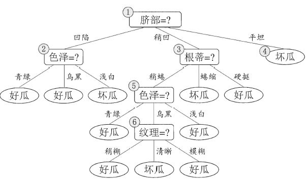
决策树的结构就像一棵树,通过不断的询问是或者否来对样本进行预测。
最开始进行分支的问题被称为根节点(root node),上图中的脐部=?就是根节点。最终的结论,也就是“好瓜”、“坏瓜”是叶子节点(leaf node)或者叫终末节点(terminal node),中间的每个问题都是中间节点。
在上下两个相邻的节点中,更靠近根节点的是父节点(parent node),另一个是子节点(child node)。
对于决策树模型来说,数据中的任何一个预测变量都可以当做是其中一个中间节点,可以不断的进行分裂,这样的好处是最终每一个样本都可以得到完美的结果,也就是误差会非常小,但是这样做一个很明显的问题就是容易使模型过拟合。
根据具体的实现方式,决策树包括多种方法,比如:ID3、C4.5、CART。
本文会介绍决策树的R语言实现和超参数调优。我会介绍决策树常见的超参数以及它们的意义,超参数调优的常见方法和调优思路,比如学习曲线、网格搜索等。
17.2 准备数据和R包
演示数据为印第安人糖尿病数据集,这个数据一共有768行,9列,其中diabetes是结果变量,为二分类,其余列是预测变量。
划分训练集、测试集。训练集用于建立模型,测试集用于测试模型表现,划分比例为7:3。
# 划分是随机的,设置种子数可以让结果复现
set.seed(123)
ind <- sample(1:nrow(pimadiabetes), size = 0.7*nrow(pimadiabetes))

# 去掉真实结果列
train <- pimadiabetes[ind,]
test <- pimadiabetes[-ind,]

dim(train)
## [1] 537   9
dim(test)
## [1] 231   9
17.3 建立模型
首先在训练集上建立模型,先不进行任何设置,就用默认的,看看效果如何:
# 决策树计算过程中有随机性,需设置种子数保证结果能复现
set.seed(123)
treefit <- rpart(diabetes ~ ., data = train)
treefit
## n= 537
##
## node), split, n, loss, yval, (yprob)
##       * denotes terminal node
##
##   1) root 537 187 pos (0.65176909 0.34823091)
##     2) insulin< 124.52 233  22 pos (0.90557940 0.09442060)
##       4) glucose< 127 210  10 pos (0.95238095 0.04761905) *
##       5) glucose>=127 23  11 neg (0.47826087 0.52173913)
##        10) mass< 34.5 15   5 pos (0.66666667 0.33333333) *
##        11) mass>=34.5 8   1 neg (0.12500000 0.87500000) *
##     3) insulin>=124.52 304 139 neg (0.45723684 0.54276316)
##       6) mass< 28.9 67  16 pos (0.76119403 0.23880597)
##        12) age< 27.5 21   1 pos (0.95238095 0.04761905) *
##        13) age>=27.5 46  15 pos (0.67391304 0.32608696)
##          26) age>=50.5 23   3 pos (0.86956522 0.13043478) *
##          27) age< 50.5 23  11 neg (0.47826087 0.52173913)
##            54) mass< 25.75 7   1 pos (0.85714286 0.14285714) *
##            55) mass>=25.75 16   5 neg (0.31250000 0.68750000) *
##       7) mass>=28.9 237  88 neg (0.37130802 0.62869198)
##        14) glucose< 158.5 182  83 neg (0.45604396 0.54395604)
##          28) age< 30.5 87  35 pos (0.59770115 0.40229885)
##            56) pressure>=73.85 45  13 pos (0.71111111 0.28888889) *
##            57) pressure< 73.85 42  20 neg (0.47619048 0.52380952)
##             114) age< 22.5 11   3 pos (0.72727273 0.27272727) *
##             115) age>=22.5 31  12 neg (0.38709677 0.61290323)
##               230) insulin< 179 20  10 pos (0.50000000 0.50000000)
##                 460) insulin>=155.66 12   4 pos (0.66666667 0.33333333) *
##                 461) insulin< 155.66 8   2 neg (0.25000000 0.75000000) *
##               231) insulin>=179 11   2 neg (0.18181818 0.81818182) *
##          29) age>=30.5 95  31 neg (0.32631579 0.67368421)
##            58) pedigree< 0.3245 33  16 pos (0.51515152 0.48484848)
##             116) insulin< 230.35 26  10 pos (0.61538462 0.38461538) *
##             117) insulin>=230.35 7   1 neg (0.14285714 0.85714286) *
##            59) pedigree>=0.3245 62  14 neg (0.22580645 0.77419355) *
##        15) glucose>=158.5 55   5 neg (0.09090909 0.90909091) *
上面就是一颗建立好的决策树,它给出了每次分支的标准。
我们可以把结果通过图形的方式画出来,默认的画图:
par(xpd = TRUE)
plot(treefit,compress = TRUE)
text(treefit, use.n = TRUE)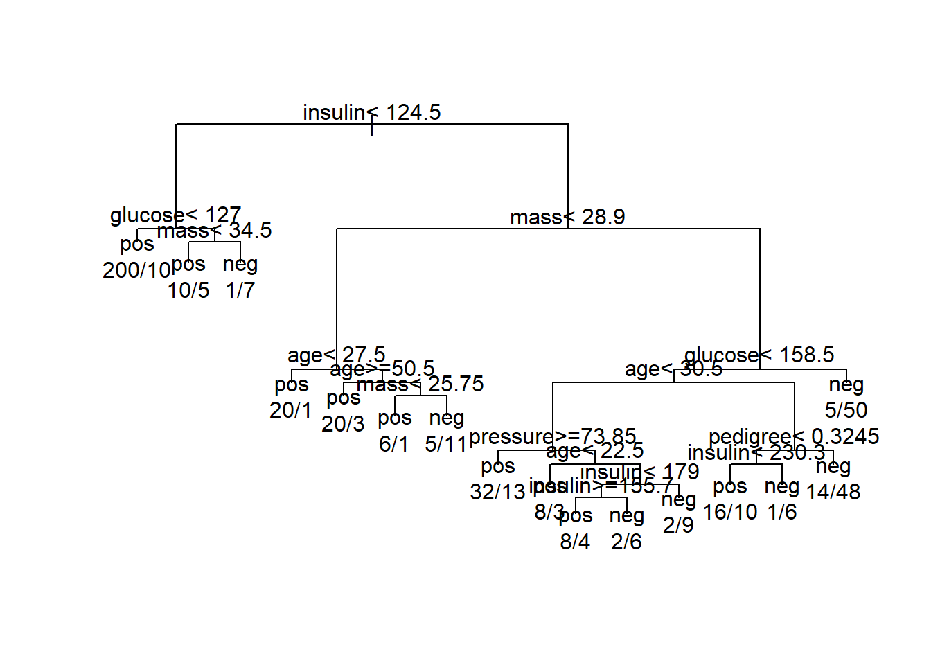
并不是很美观,建立好的决策树的结果还可以通过rpart.plot函数画出来:
rpart.plot(treefit)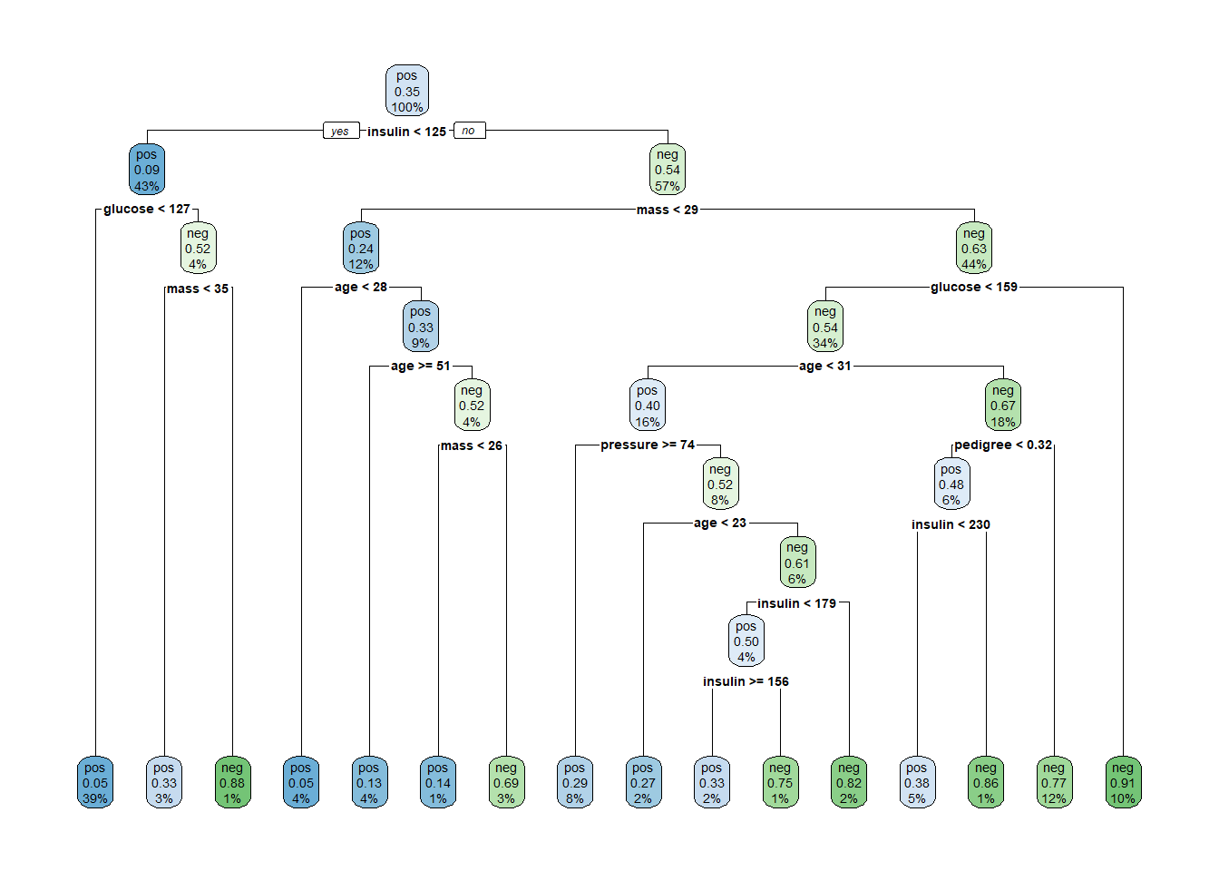
这样的结果一目了然,它告诉我们,第一次分支使用了insulin这个变量,分支的标准是124.5,分支后每个子节点的样本比例也很清楚的显示了。
这棵树一共分支了8次,树的深度为9层。
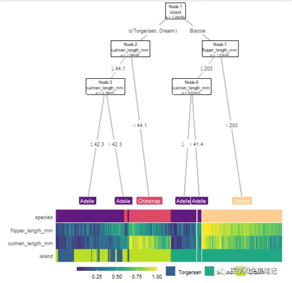
也可以使用partykit进行可视化:
library(partykit)

plot(as.party(treefit))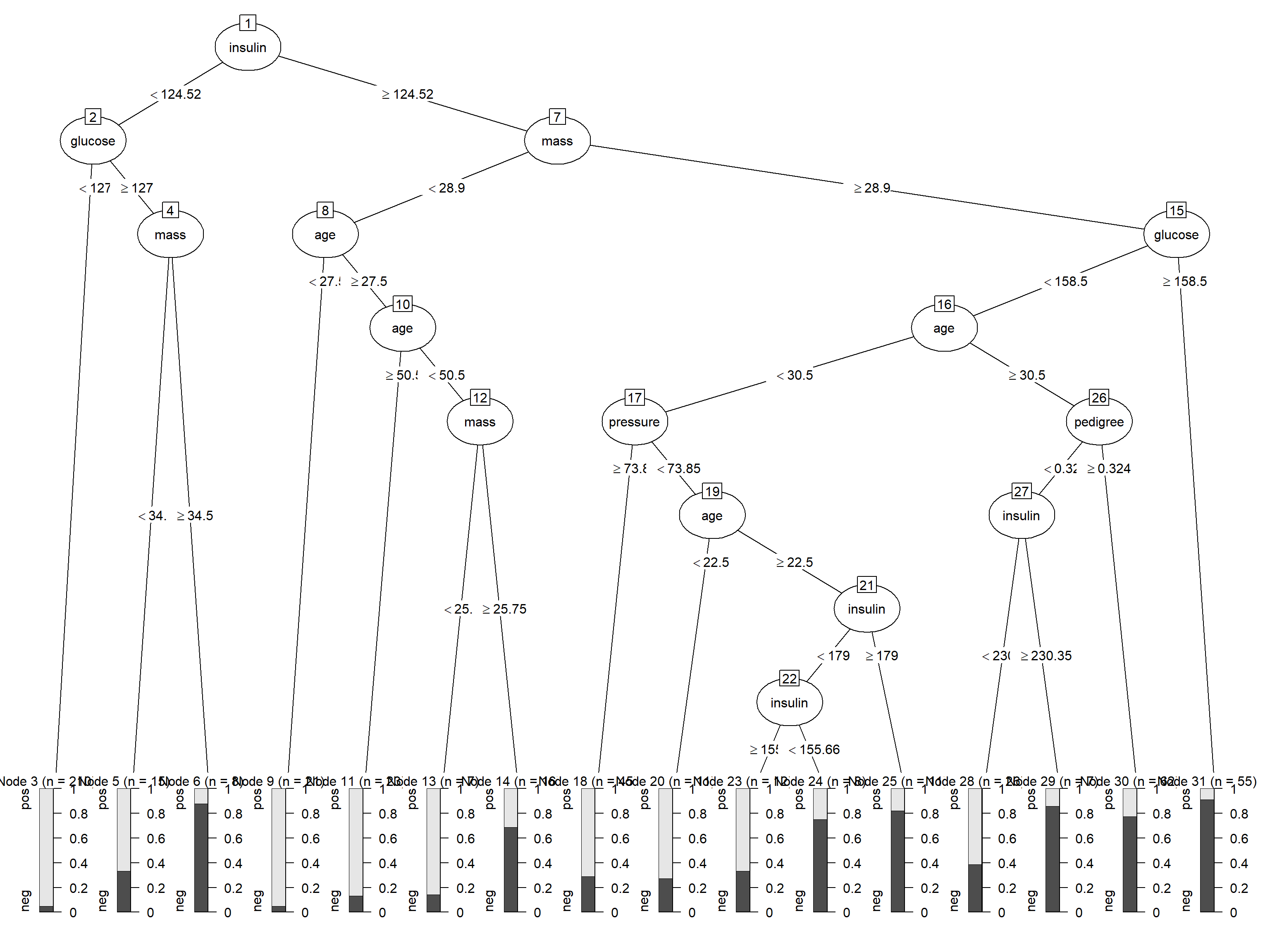
如果你还想要更加花里胡哨的可视化效果,可以试一下我们之前介绍过的treeheatR,效果绝对炫酷:超级炫酷的决策树可视化R包
17.4 超参数介绍
这是默认情况下建立好的决策树,没有进行任何的超参数调优,这样的一棵树,会自由地“生长”,直到不能再生长为止。
决策树的超参数有很多,大部分都是和剪枝有关的,通过剪枝参数,可以有效限制树的生长(防止过拟合),这几个参数也是所有和树有关的模型的通用参数,比如随机森林,常见的有:
- 树的深度:设置树分支的最大深度;
- 使用的特征个数:设置建立模型时最多使用几个特征;
- 最小分支节点:如果当前节点的样本数少于某个值就不再往下分支了。
常见的是这几个,其他还有很多,需要深入了解可以自行学习。
这些超参数都可以通过rpart.control函数设置。
通过预先设定好这些参数的值,达到防止树过度生长的目的,这种叫做预剪枝。
除此之外,rpart.control函数中提供了cp参数,可以用来实现后剪枝。
当决策树复杂度超过一定程度后,随着复杂度的提高,模型的分类准确度反而会降低。因此,建立的决策树不宜太复杂,需进行剪枝。该剪枝算法依赖于复杂度参数cp,cp随树复杂度的增加而减小,当增加一个节点引起的分类准确度变化量小于树复杂度变化的cp倍时,则须剪去该节点。故建立一棵既能精确分类,又不过度拟合的决策树的关键是求解一个合适的cp值。一般选择错判率最小值(Xerror)对应的cp值来修剪。
rpart函数默认是使用十折交叉验证进行计算,也可以通过rpart.control函数进行设置
# 这里都选择了默认值

set.seed(123)
treefit <- rpart(diabetes ~ ., data = train,
                 control = rpart.control(minsplit = 20, # 最小分支节点
                                         #minbucket = 2, # 分支后最小节点
                                         maxdepth = 30, # 树的深度
                                         cp = 0.01, # 复杂度
                                         xval = 10 # 交叉验证,默认10折
                                         )
                 )
treefit
## n= 537
##
## node), split, n, loss, yval, (yprob)
##       * denotes terminal node
##
##   1) root 537 187 pos (0.65176909 0.34823091)
##     2) insulin< 124.52 233  22 pos (0.90557940 0.09442060)
##       4) glucose< 127 210  10 pos (0.95238095 0.04761905) *
##       5) glucose>=127 23  11 neg (0.47826087 0.52173913)
##        10) mass< 34.5 15   5 pos (0.66666667 0.33333333) *
##        11) mass>=34.5 8   1 neg (0.12500000 0.87500000) *
##     3) insulin>=124.52 304 139 neg (0.45723684 0.54276316)
##       6) mass< 28.9 67  16 pos (0.76119403 0.23880597)
##        12) age< 27.5 21   1 pos (0.95238095 0.04761905) *
##        13) age>=27.5 46  15 pos (0.67391304 0.32608696)
##          26) age>=50.5 23   3 pos (0.86956522 0.13043478) *
##          27) age< 50.5 23  11 neg (0.47826087 0.52173913)
##            54) mass< 25.75 7   1 pos (0.85714286 0.14285714) *
##            55) mass>=25.75 16   5 neg (0.31250000 0.68750000) *
##       7) mass>=28.9 237  88 neg (0.37130802 0.62869198)
##        14) glucose< 158.5 182  83 neg (0.45604396 0.54395604)
##          28) age< 30.5 87  35 pos (0.59770115 0.40229885)
##            56) pressure>=73.85 45  13 pos (0.71111111 0.28888889) *
##            57) pressure< 73.85 42  20 neg (0.47619048 0.52380952)
##             114) age< 22.5 11   3 pos (0.72727273 0.27272727) *
##             115) age>=22.5 31  12 neg (0.38709677 0.61290323)
##               230) insulin< 179 20  10 pos (0.50000000 0.50000000)
##                 460) insulin>=155.66 12   4 pos (0.66666667 0.33333333) *
##                 461) insulin< 155.66 8   2 neg (0.25000000 0.75000000) *
##               231) insulin>=179 11   2 neg (0.18181818 0.81818182) *
##          29) age>=30.5 95  31 neg (0.32631579 0.67368421)
##            58) pedigree< 0.3245 33  16 pos (0.51515152 0.48484848)
##             116) insulin< 230.35 26  10 pos (0.61538462 0.38461538) *
##             117) insulin>=230.35 7   1 neg (0.14285714 0.85714286) *
##            59) pedigree>=0.3245 62  14 neg (0.22580645 0.77419355) *
##        15) glucose>=158.5 55   5 neg (0.09090909 0.90909091) *
可以看到这棵树和我们最开始建立的模型一模一样,因为我们用了默认的设置,并没有更改。
接下来我们在测试集上看看模型表现:
pred <- predict(treefit, newdata = test,type = "class")

# 计算混淆矩阵
caret::confusionMatrix(test$diabetes, pred)
## Confusion Matrix and Statistics
##
##           Reference
## Prediction pos neg
##        pos 130  20
##        neg  36  45
##
##                Accuracy : 0.7576
##                  95% CI : (0.697, 0.8114)
##     No Information Rate : 0.7186
##     P-Value [Acc > NIR] : 0.10561
##
##                   Kappa : 0.4423
##
##  Mcnemar's Test P-Value : 0.04502
##
##             Sensitivity : 0.7831
##             Specificity : 0.6923
##          Pos Pred Value : 0.8667
##          Neg Pred Value : 0.5556
##              Prevalence : 0.7186
##          Detection Rate : 0.5628
##    Detection Prevalence : 0.6494
##       Balanced Accuracy : 0.7377
##
##        'Positive' Class : pos
##
混淆矩阵的结果显示准确度Accuracy : 0.6987,效果不是很好!
17.5 后剪枝
下面我们通过cp参数进行后剪枝。
首先可以通过printcp函数查看复杂度和误差之间的数值关系:
printcp(treefit)
##
## Classification tree:
## rpart(formula = diabetes ~ ., data = train, control = rpart.control(minsplit = 20,
##     maxdepth = 30, cp = 0.01, xval = 10))
##
## Variables actually used in tree construction:
## [1] age      glucose  insulin  mass     pedigree pressure
##
## Root node error: 187/537 = 0.34823
##
## n= 537
##
##         CP nsplit rel error  xerror     xstd
## 1 0.163102      0   1.00000 1.00000 0.059037
## 2 0.045455      2   0.67380 0.82353 0.056044
## 3 0.018717      4   0.58289 0.71658 0.053626
## 4 0.016043      6   0.54545 0.66310 0.052222
## 5 0.010695     10   0.48128 0.67380 0.052514
## 6 0.010000 15 0.42781 0.66845 0.052369CP是复杂度参数,nsplit是分裂次数,rel error是相对误差,即某次分裂的RSS(残差平方和)除以不分裂的RSS,xerror是平均误差,xstd是交叉验证的标准差
从上面的结果可以看出,CP=0.016043时,分裂次数为6,平均误差和标准差最小,分别是0.66310和0.052222。
下面用图形化的方式展示结果:
plotcp(treefit)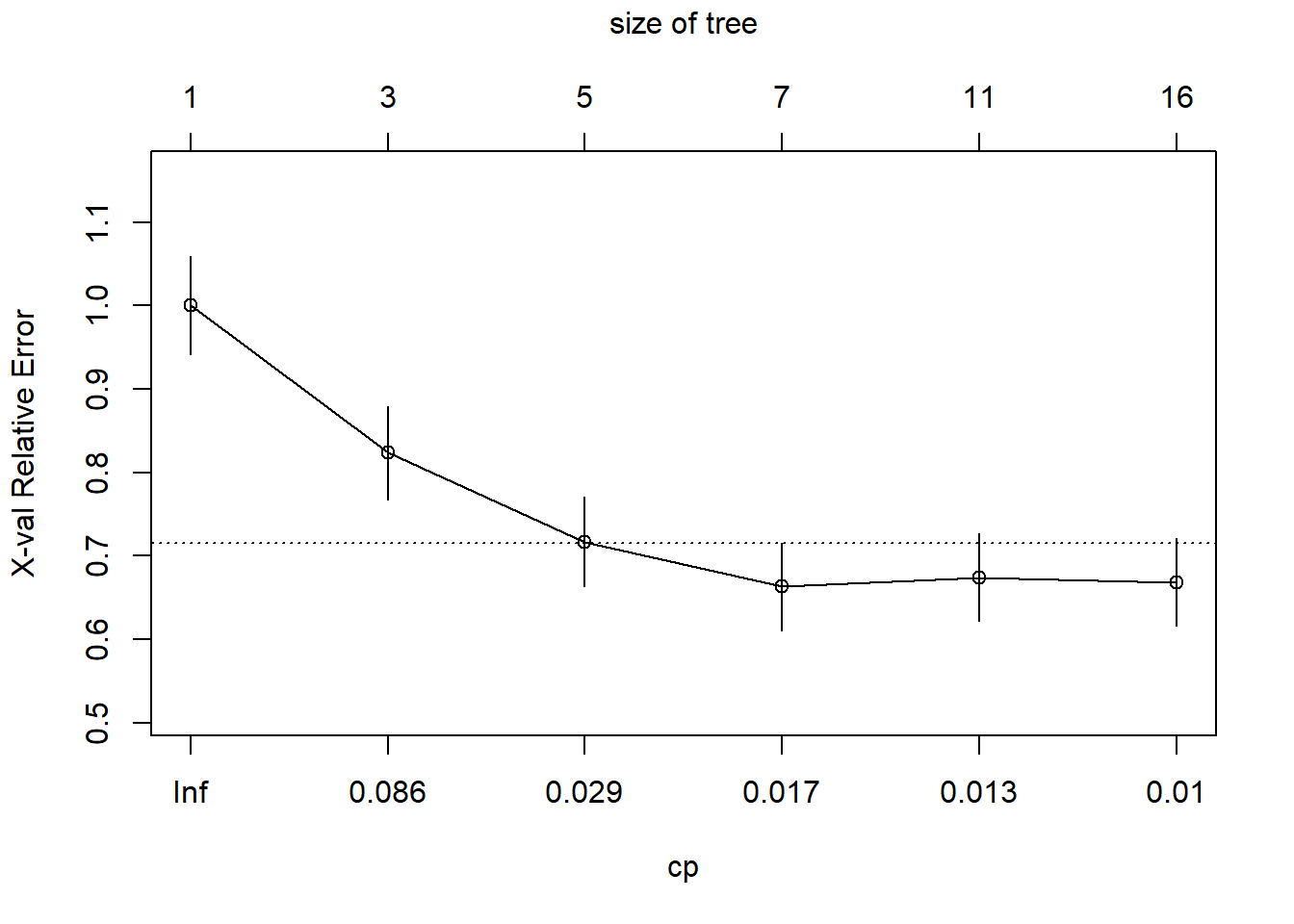
纵坐标是相对误差,底下的横坐标是复杂度,上面的横坐标是树的规模,上面可以看出树的规模为7(也就是分裂6次)时,相对误差最小,和上面printcp()结果相同。
接下来就可以就可以根据CP进行剪枝了,通常选择xerror最小时的CP值(还有别的选择方法,比如1倍标准差法等):
cp <- treefit$cptable[which.min(treefit$cptable[,"xerror"]), "CP"]
cp
## [1] 0.01604278
treepruned <- prune(treefit, cp = cp)
treepruned
## n= 537
##
## node), split, n, loss, yval, (yprob)
##       * denotes terminal node
##
##   1) root 537 187 pos (0.65176909 0.34823091)
##     2) insulin< 124.52 233  22 pos (0.90557940 0.09442060) *
##     3) insulin>=124.52 304 139 neg (0.45723684 0.54276316)
##       6) mass< 28.9 67  16 pos (0.76119403 0.23880597) *
##       7) mass>=28.9 237  88 neg (0.37130802 0.62869198)
##        14) glucose< 158.5 182  83 neg (0.45604396 0.54395604)
##          28) age< 30.5 87  35 pos (0.59770115 0.40229885)
##            56) pressure>=73.85 45  13 pos (0.71111111 0.28888889) *
##            57) pressure< 73.85 42  20 neg (0.47619048 0.52380952)
##             114) age< 22.5 11   3 pos (0.72727273 0.27272727) *
##             115) age>=22.5 31  12 neg (0.38709677 0.61290323) *
##          29) age>=30.5 95  31 neg (0.32631579 0.67368421) *
##        15) glucose>=158.5 55   5 neg (0.09090909 0.90909091) *
剪枝后的树简单多了,画图展示剪枝后的树:
rpart.plot(treepruned)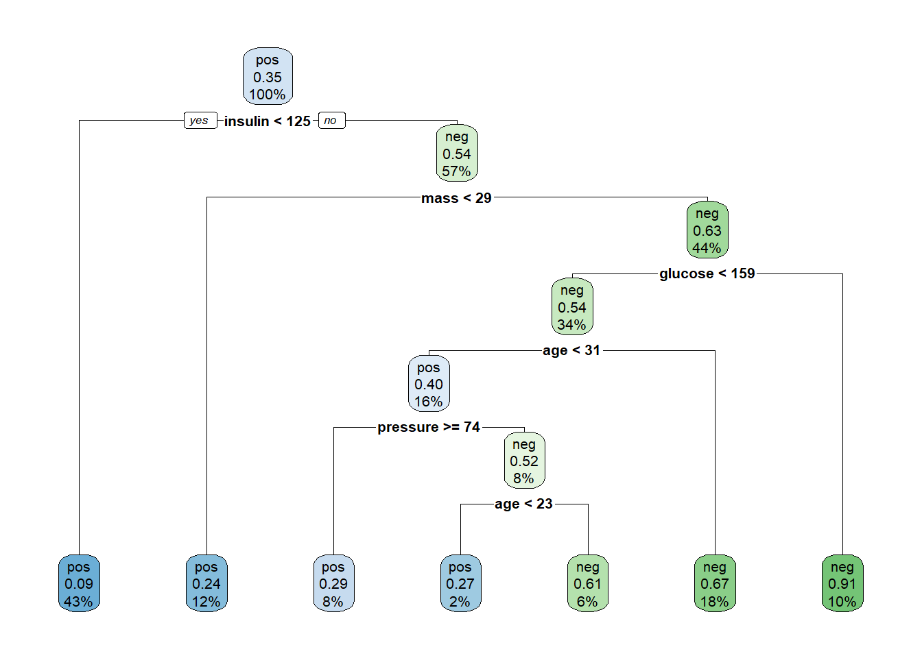
接下来使用修剪后的树再次作用于测试集:
pred2 <- predict(treepruned, newdata = test, type = "class")
caret::confusionMatrix(test$diabetes, pred2)
## Confusion Matrix and Statistics
##
##           Reference
## Prediction pos neg
##        pos 120  30
##        neg  26  55
##
##                Accuracy : 0.7576
##                  95% CI : (0.697, 0.8114)
##     No Information Rate : 0.632
##     P-Value [Acc > NIR] : 3.133e-05
##
##                   Kappa : 0.4736
##
##  Mcnemar's Test P-Value : 0.6885
##
##             Sensitivity : 0.8219
##             Specificity : 0.6471
##          Pos Pred Value : 0.8000
##          Neg Pred Value : 0.6790
##              Prevalence : 0.6320
##          Detection Rate : 0.5195
##    Detection Prevalence : 0.6494
##       Balanced Accuracy : 0.7345
##
##        'Positive' Class : pos
##
通过后剪枝的准确度和不剪枝的结果差不多,但是由于分裂次数明显减少,模型复杂度明显减小了。
这是非常常见的情况,有时候你调优后的模型可能还不如默认的好,有时候却效果超群,原因是多方面的,首先是数据问题,其次是选择的方法。
17.6 学习曲线
接下来我们看看通过预剪枝能不能让模型的表现更好一点。
如果要对单个超参数进行调优,我们可以用学习曲线的方式,学习曲线的横坐标是超参数的各个取值,纵坐标是不同超参数下的模型表现,通过学习曲线,可以找到模型表现较好的超参数值。
我们就以调整minsplit为例。
minsplit是每个节点的最少样本量,我们训练集一共有537个样本,就设置为2:300先看看情况。
模型的评价指标选择准确率。
res <- list()
for(i in 2:300){

  f <- rpart(diabetes ~ ., data = train,
                 control = rpart.control(minsplit = i )
             )
  pred <- predict(f, newdata = test,type = "class")
  acc <- caret::confusionMatrix(test$diabetes, pred)[["overall"]][["Accuracy"]]
  df <- data.frame(minsplit = i, accuracy = acc)
  res[[i-1]] <- df
}

acc.res <- do.call(rbind, res)
查看准确率的范围:
range(acc.res$accuracy)
## [1] 0.6969697 0.7878788
准确率最高是0.7878788,接下来我们把结果画出来:
library(ggplot2)

ggplot(acc.res, aes(minsplit, accuracy))+
  geom_point()+
  geom_line()+
  geom_vline(xintercept = 13,linetype = 2, color = "red")+
  theme_bw()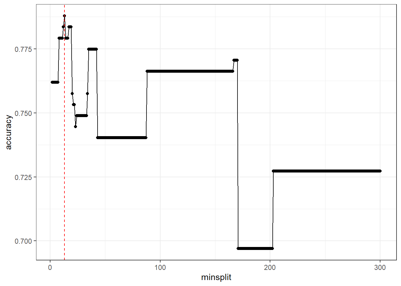
这个图就是minsplit的学习曲线,从这个学习曲线可以看出,minsplit=13的时候,准确度accuracy达到了最大。
我们可以轻松找出准确度最高的minsplit值(可能有多个minsplit都对应着最高的准确率,但是我们肯定是优先选择最简单的一个):
acc.res[which.max(acc.res$accuracy),]
##    minsplit  accuracy
## 12 13 0.7878788minsplit为13时,准确度就已经到最高了。这个结果比后剪枝的结果好一点。
所以我们就选择minsplit为13,重新建立决策树模型。
# 建立模型
set.seed(123)
treef <- rpart(diabetes ~ ., data = train,
               control = rpart.control(minsplit = 13) # 这里选择13
               )

# 测试集查看效果
pred <- predict(treef, newdata = test,type = "class")

# 测试集的混淆矩阵
caret::confusionMatrix(test$diabetes, pred)
## Confusion Matrix and Statistics
##
##           Reference
## Prediction pos neg
##        pos 126  24
##        neg  25  56
##
##                Accuracy : 0.7879
##                  95% CI : (0.7295, 0.8388)
##     No Information Rate : 0.6537
##     P-Value [Acc > NIR] : 5.953e-06
##
##                   Kappa : 0.5329
##
##  Mcnemar's Test P-Value : 1
##
##             Sensitivity : 0.8344
##             Specificity : 0.7000
##          Pos Pred Value : 0.8400
##          Neg Pred Value : 0.6914
##              Prevalence : 0.6537
##          Detection Rate : 0.5455
##    Detection Prevalence : 0.6494
##       Balanced Accuracy : 0.7672
##
##        'Positive' Class : pos
##
决策树的可视化:
rpart.plot(treef)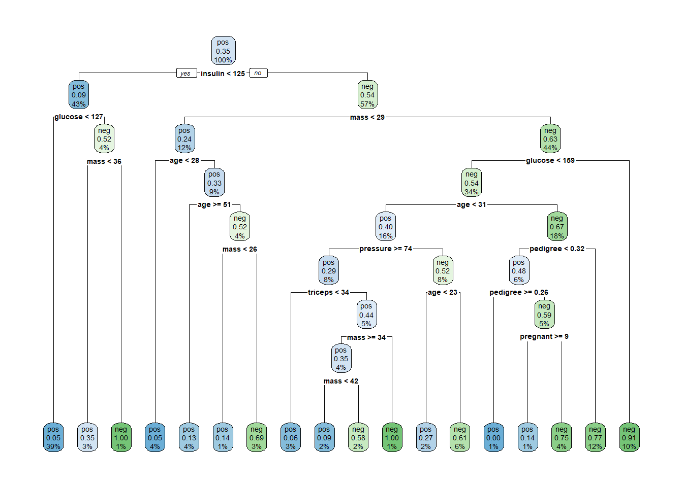
17.7 网格搜索
学习曲线适合于某个单独的超参数调优,如果是多个超参数一起调优还是要使用其他方法,最常见的一种就是网格搜索,网格搜索现在我们有非常成熟的工具包,比如tidymodels、mlr3、caret。
但是今天我想介绍下使用e1071包实现网格搜索,这个包功能强大,不仅可以实现支持向量机,而且包含多种调优功能,详情请参考:R语言支持向量机e1071
library(e1071)

# 默认10折交叉验证
set.seed(456)
tune_obj <- tune.rpart(diabetes ~ ., data = train,
                       minsplit = seq(10,120,5),
                       cp = c(0.0001,0.001,0.01,0.1,1)
                       )

tune_obj
##
## Parameter tuning of 'rpart.wrapper':
##
## - sampling method: 10-fold cross validation
##
## - best parameters:
##  minsplit    cp
##       100 1e-04
##
## - best performance: 0.2269392速度很快,使用也很简单。直接给出最优结果是minsplit=100,cp=0.0001。
重新拟合模型:
rpart_fit <- rpart(diabetes ~ ., data = train,
                   control = rpart.control(minsplit = 100,
                                         cp = 0.0001,
                                         xval = 10
                                         )
                   )
rpart_fit
## n= 537
##
## node), split, n, loss, yval, (yprob)
##       * denotes terminal node
##
##  1) root 537 187 pos (0.65176909 0.34823091)
##    2) insulin< 124.52 233  22 pos (0.90557940 0.09442060) *
##    3) insulin>=124.52 304 139 neg (0.45723684 0.54276316)
##      6) mass< 28.9 67  16 pos (0.76119403 0.23880597) *
##      7) mass>=28.9 237  88 neg (0.37130802 0.62869198)
##       14) glucose< 158.5 182  83 neg (0.45604396 0.54395604)
##         28) age< 30.5 87  35 pos (0.59770115 0.40229885) *
##         29) age>=30.5 95  31 neg (0.32631579 0.67368421) *
##       15) glucose>=158.5 55   5 neg (0.09090909 0.90909091) *
这棵树就简单多了,效果也不错。
接下来我们在测试集上看看模型表现:
pred <- predict(rpart_fit, newdata = test,type = "class")

# 计算混淆矩阵
caret::confusionMatrix(test$diabetes, pred)
## Confusion Matrix and Statistics
##
##           Reference
## Prediction pos neg
##        pos 128  22
##        neg  32  49
##
##                Accuracy : 0.7662
##                  95% CI : (0.7063, 0.8192)
##     No Information Rate : 0.6926
##     P-Value [Acc > NIR] : 0.00816
##
##                   Kappa : 0.4717
##
##  Mcnemar's Test P-Value : 0.22067
##
##             Sensitivity : 0.8000
##             Specificity : 0.6901
##          Pos Pred Value : 0.8533
##          Neg Pred Value : 0.6049
##              Prevalence : 0.6926
##          Detection Rate : 0.5541
##    Detection Prevalence : 0.6494
##       Balanced Accuracy : 0.7451
##
##        'Positive' Class : pos
##
混淆矩阵的结果显示准确度Accuracy : 0.7662 ,效果还可以哦!