rm(list = ls())
library(randomForest)

load(file = "datasets/pimadiabetes.rdata")

dim(pimadiabetes)
## [1] 768   9
str(pimadiabetes)
## 'data.frame':    768 obs. of  9 variables:
##  $ pregnant: num  6 1 8 1 0 5 3 10 2 8 ...
##  $ glucose : num  148 85 183 89 137 116 78 115 197 125 ...
##  $ pressure: num  72 66 64 66 40 ...
##  $ triceps : num  35 29 22.9 23 35 ...
##  $ insulin : num  202.2 64.6 217.1 94 168 ...
##  $ mass    : num  33.6 26.6 23.3 28.1 43.1 ...
##  $ pedigree: num  0.627 0.351 0.672 0.167 2.288 ...
##  $ age     : num  50 31 32 21 33 30 26 29 53 54 ...
## $ diabetes: Factor w/ 2 levels "pos","neg": 2 1 2 1 2 1 2 1 2 2 ...20 随机森林
随机森林是一种集成(ensemble)算法,属于集成算法中的袋装法(bagging)。随机森林可以生成多棵树(决策树)模型,然后将这些树的结果组合起来。
随机森林在建立模型时,会使用自助法(bootstrap)进行重抽样,每次使用大概全部观测的2/3拟合模型,在剩下的1/3的观测中衡量模型性能,这剩下的1/3的数据就被称为袋外数据(out-of-bag),对袋外数据进行的预测就叫袋外预测(out-of-bag prediction),或者叫样本外预测(out-of-sample prediction)。这个过程会重复几十或者几百次,最后取平均结果。
随机森林支持分类、回归、生存分析等多种任务类型,而且对数据的要求不严格,即使不进行预处理也能直接使用(但是不能有缺失值)。
目前R语言做随机森林主要就是ranger和randomForest包。ranger的开发者就是survivalsvm的开发者。ranger是使用c++实现的,速度超快。
但是ranger的相关文档太少了,而且缺少可视化函数,我们主要介绍randomForest。
20.1 加载R包和数据
演示数据为印第安人糖尿病数据集,这个数据一共有768行,9列,其中diabetes是结果变量,为二分类,其余列是预测变量。
20.2 数据划分
划分训练集、测试集。训练集用于建立模型,测试集用于测试模型表现,划分比例为7:3。
# 划分是随机的,设置种子数可以让结果复现
set.seed(123)
ind <- sample(1:nrow(pimadiabetes), size = 0.7*nrow(pimadiabetes))

# 去掉真实结果列
train <- pimadiabetes[ind,]
test <- pimadiabetes[-ind,]

dim(train)
## [1] 537   9
dim(test)
## [1] 231   9
20.3 建立模型
在训练集拟合模型,参数importance=T表示需要计算变量的重要性:
set.seed(123)
fit <- randomForest(diabetes ~ ., data = train, importance = T)
fit
##
## Call:
##  randomForest(formula = diabetes ~ ., data = train, importance = T)
##                Type of random forest: classification
##                      Number of trees: 500
## No. of variables tried at each split: 2
##
##         OOB estimate of  error rate: 22.91%
## Confusion matrix:
##     pos neg class.error
## pos 299  51   0.1457143
## neg  72 115   0.3850267
结果给出了树的数量:500颗;OOB错误率;还给出了混淆矩阵。
20.4 结果探索
下面是可视化整体错误率和树的数量的关系,可以看到随着树的数量增加,错误率逐渐降低并渐趋平稳,中间的黑色线条是整体的错误率,上下两条是结果变量中两个类别的错误率。
plot(fit)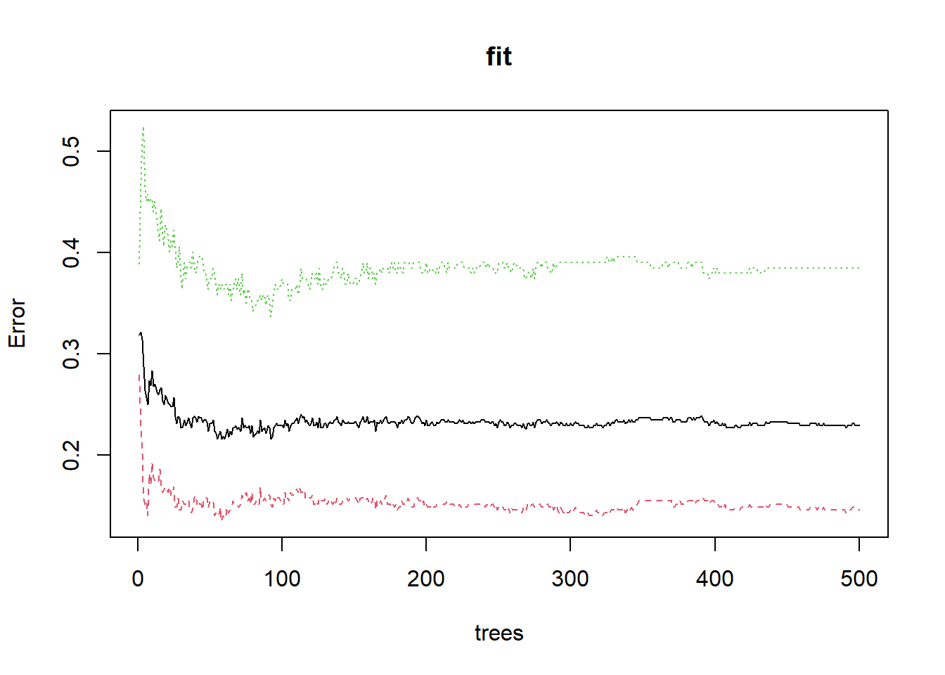
查看整体错误率最小时有几棵树:
which.min(fit$err.rate[,1])
## [1] 55查看各个变量的重要性,这里还给出了mean decrease gini,数值越大说明变量越重要:
randomForest::importance(fit)
##                pos       neg MeanDecreaseAccuracy MeanDecreaseGini
## pregnant  3.076717  2.318634            4.0433361         15.45065
## glucose  26.966011 22.856482           35.5073316         52.00314
## pressure  1.148162 -0.574716            0.4489352         17.98889
## triceps   7.448920  3.465856            8.4222497         24.27110
## insulin  20.385928 20.507513           29.5489019         50.91964
## mass      8.257001 18.574513           18.9842081         34.35775
## pedigree  5.186099  4.690982            6.9584762         24.19246
## age       6.456647  7.064110            9.6989105         23.94584
可视化变量重要性:
varImpPlot(fit)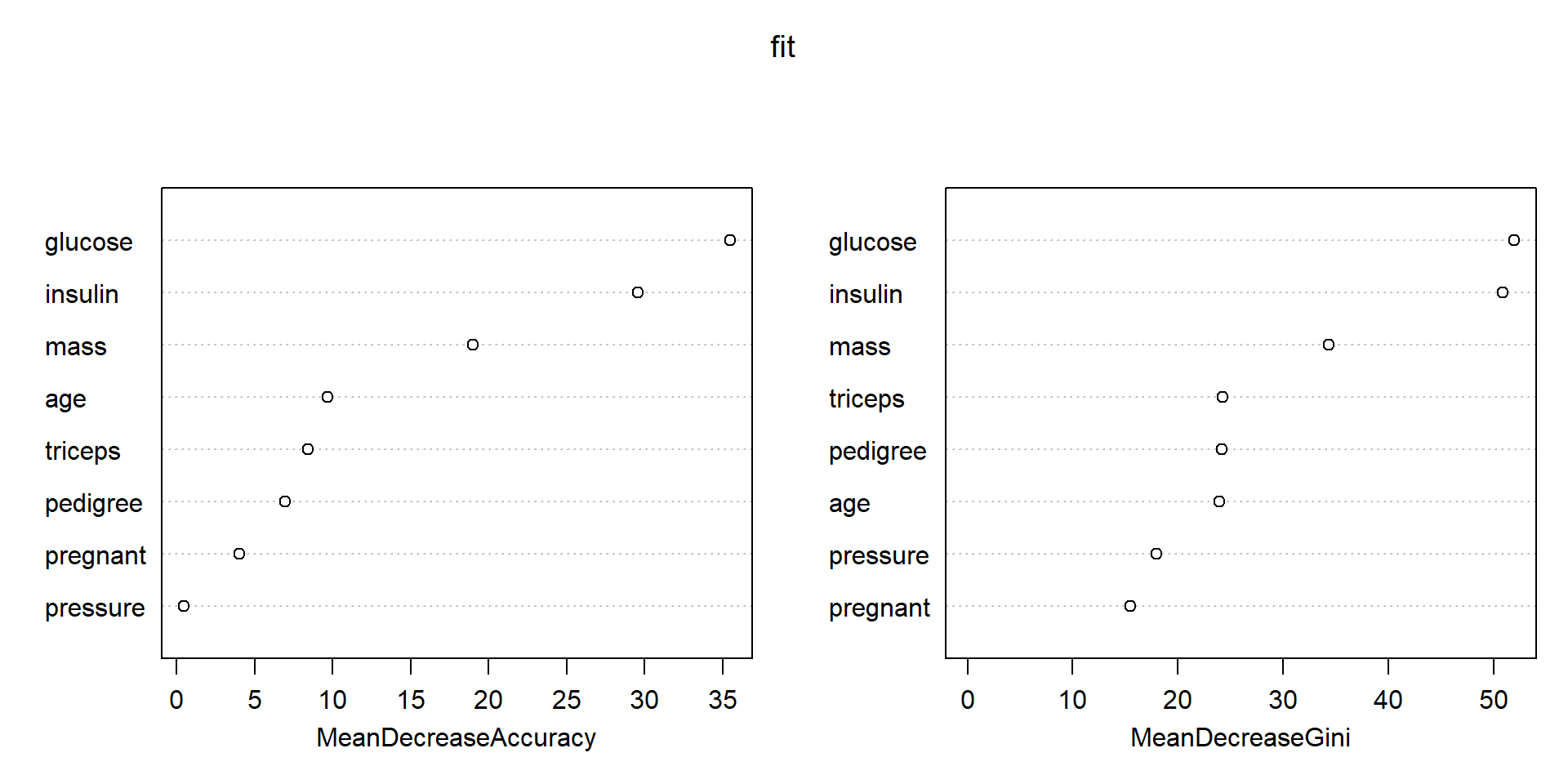
通过变量重要性,大家就可以选择比较重要的变量了。你可以选择前5个,前10个,或者大于所有变量重要性平均值(中位数,百分位数等)的变量等等。
使用随机森林筛选变量,我专门写过一篇文章:R语言随机森林筛选变量
这个图还可以使用ggRandomForests来画,更加好看:
library(ggRandomForests)
gg_dta <- gg_vimp(fit)
plot(gg_dta) #MeanDecreaseGini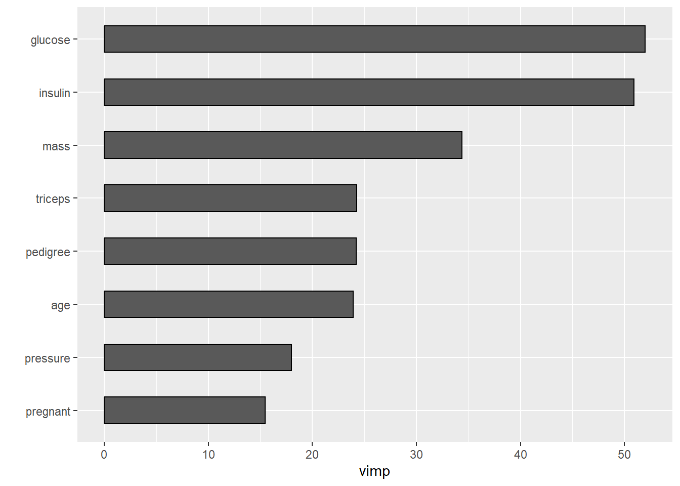
或者通过vip来画:
library(vip)

vip(fit) #MeanDecreaseAccuracy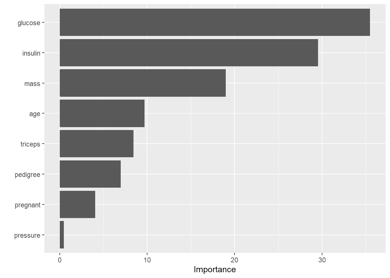
20.4.1 提取某一棵树
会给出这颗树在分支时的各种细节,结果太长了,没放出来:
getTree(fit, k=2)20.4.2 重新建立模型
选择树的数量为55,并重新建立模型:
fit1 <- randomForest(diabetes ~ ., data = train, ntree = 55)
fit1
##
## Call:
##  randomForest(formula = diabetes ~ ., data = train, ntree = 55)
##                Type of random forest: classification
##                      Number of trees: 55
## No. of variables tried at each split: 2
##
##         OOB estimate of  error rate: 24.02%
## Confusion matrix:
##     pos neg class.error
## pos 299  51   0.1457143
## neg  78 109   0.4171123
查看测试集效果:
pred <- predict(fit1, newdata = test)
head(pred)
##   1   3   4   9  15  17
## neg neg pos neg pos neg
## Levels: pos neg
混淆矩阵:
caret::confusionMatrix(test$diabetes, pred)
## Confusion Matrix and Statistics
##
##           Reference
## Prediction pos neg
##        pos 127  23
##        neg  33  48
##
##                Accuracy : 0.7576
##                  95% CI : (0.697, 0.8114)
##     No Information Rate : 0.6926
##     P-Value [Acc > NIR] : 0.01776
##
##                   Kappa : 0.4521
##
##  Mcnemar's Test P-Value : 0.22910
##
##             Sensitivity : 0.7937
##             Specificity : 0.6761
##          Pos Pred Value : 0.8467
##          Neg Pred Value : 0.5926
##              Prevalence : 0.6926
##          Detection Rate : 0.5498
##    Detection Prevalence : 0.6494
##       Balanced Accuracy : 0.7349
##
##        'Positive' Class : pos
##
准确率0.7576,效果一般。
# 计算预测概率,准备绘制ROC曲线
pred <- predict(fit1, newdata = test, type = "prob")
head(pred)
##          pos       neg
## 1  0.3454545 0.6545455
## 3  0.4181818 0.5818182
## 4  1.0000000 0.0000000
## 9  0.1454545 0.8545455
## 15 0.6181818 0.3818182
## 17 0.3272727 0.6727273
ROC曲线:
library(pROC)

# 提供真实结果,预测概率
rocc <- roc(test$diabetes, as.matrix(pred)[,1])
rocc
##
## Call:
## roc.default(response = test$diabetes, predictor = as.matrix(pred)[,     1])
##
## Data: as.matrix(pred)[, 1] in 150 controls (test$diabetes pos) > 81 cases (test$diabetes neg).
## Area under the curve: 0.8438

plot(rocc,
     print.auc=TRUE,
     auc.polygon=TRUE,
     max.auc.polygon=TRUE,
     auc.polygon.col="skyblue",
     grid=c(0.1, 0.2),
     grid.col=c("green", "red"),
     print.thres=TRUE)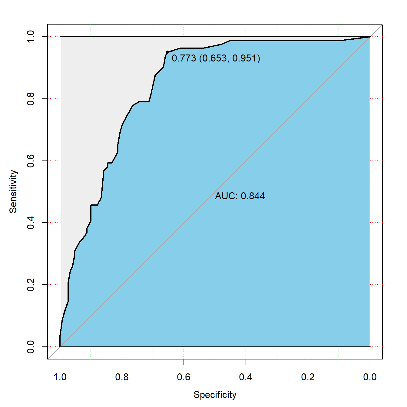
训练集的ROC曲线怎么画呢?
# 也是先计算预测概率
pred_train <- predict(fit1, newdata = train, type = "prob")

library(pROC)
# 提供真实结果,预测概率
rocc <- roc(train$diabetes, as.matrix(pred_train)[,1])
rocc
##
## Call:
## roc.default(response = train$diabetes, predictor = as.matrix(pred_train)[,     1])
##
## Data: as.matrix(pred_train)[, 1] in 350 controls (train$diabetes pos) > 187 cases (train$diabetes neg).
## Area under the curve: 1

plot(rocc,
     print.auc=TRUE,
     auc.polygon=TRUE,
     max.auc.polygon=TRUE,
     auc.polygon.col="skyblue",
     grid=c(0.1, 0.2),
     grid.col=c("green", "red"),
     print.thres=TRUE)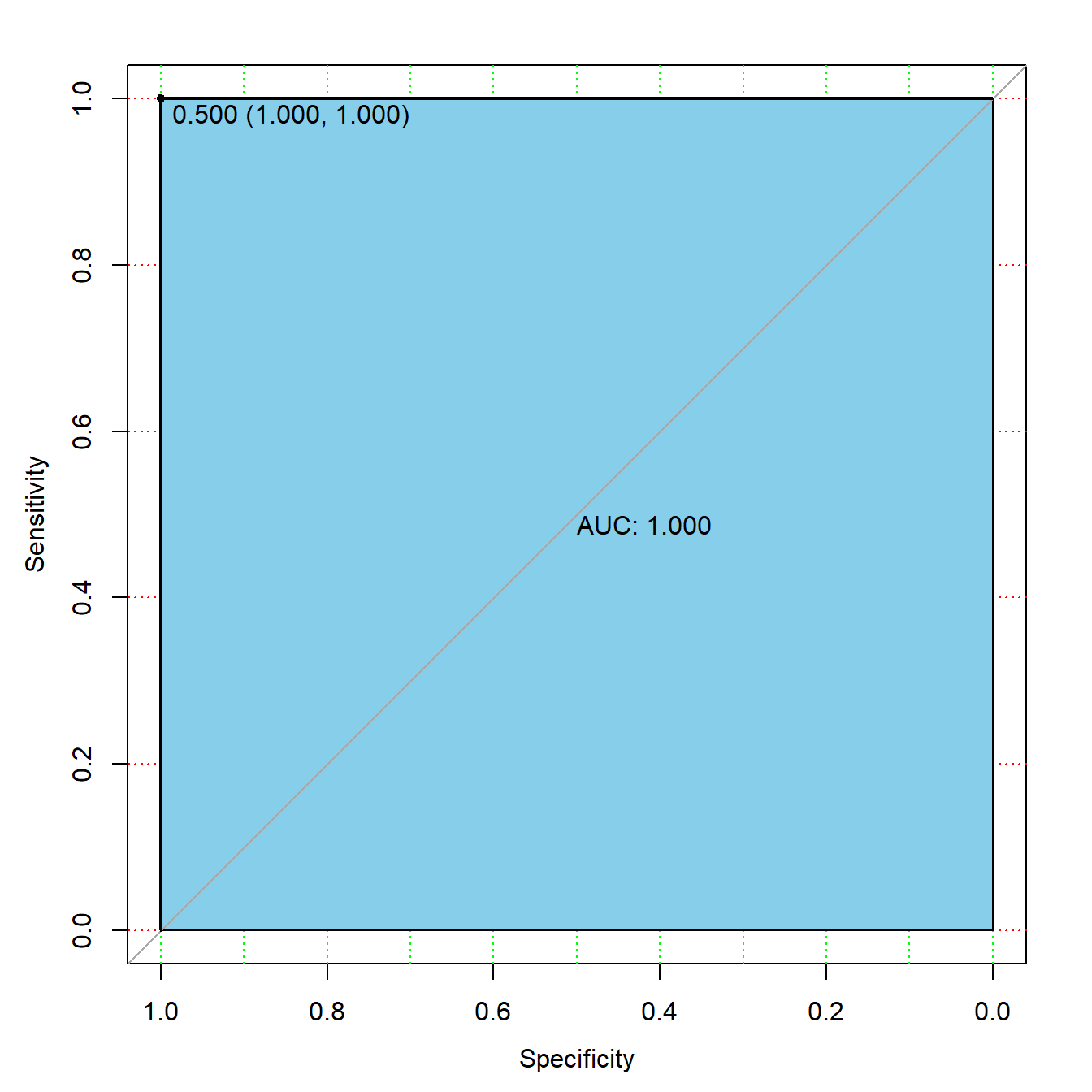
训练集的AUC是1,但测试集的AUC只有0.84,严重的过拟合,随机森林本身就是容易过拟合的模型,它的各种超参数也都是降低模型复杂度,防止过拟合的。
随机森林的网格搜索超参数调优可以通过caret、mlr3、tidymodels实现,caret法之前已介绍过,可参考:R语言机器学习caret-10:随机森林的小例子
20.5 超参数调优
randomForest自带一个调优函数:tuneRF(),可以实现对mtry的调优:
#?tuneRF
tuneRF(x = train[,-9], y = train$diabetes)
## mtry = 2  OOB error = 26.82%
## Searching left ...
## mtry = 1     OOB error = 24.02%
## 0.1041667 0.05
## Searching right ...
## mtry = 4     OOB error = 24.21%
## -0.007751938 0.05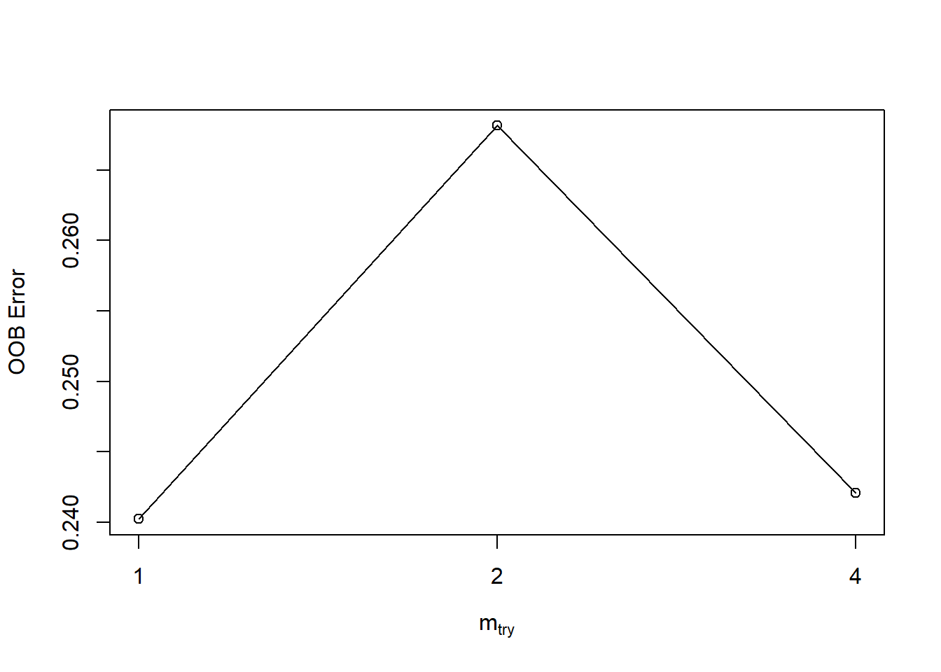
##       mtry  OOBError
## 1.OOB    1 0.2402235
## 2.OOB    2 0.2681564
## 4.OOB    4 0.2420857
结果如上图。
轻量化的调参我还是推荐使用e1071包实现。
其中的tune.randomForest()可实现对随机森林中mtry、nodesize、ntree3个超参数的调节,默认使用10折交叉验证法。
mtry:每次分支时使用的预测变量数量,肯定是介于 1个~预测变量个数,之间nodesize:终末节点的样本量,如果这个数量特别大,那肯定树的深度就不会很深,可以防止过拟合ntree:使用的树的数量,对于随机森林来说这个数量肯定是越多越好,通常选500或1000
library(e1071)

tune_res <- tune.randomForest(x = train[,-9], y = train$diabetes,
                  nodesize = c(1:3),
                  mtry = c(2,4,6,8),
                  ntree = 500
                  )
#save(tune_res,file = "datasets/tune_res.rdata")load(file = "datasets/tune_res.rdata")
tune_res
##
## Parameter tuning of 'randomForest':
##
## - sampling method: 10-fold cross validation
##
## - best parameters:
## nodesize mtry ntree
## 3 5 500
##
## - best performance: 0.06731802查看错误率:
tune_res$performances
##   nodesize mtry ntree      error  dispersion
## 1        1    2   500 0.07100520 0.003384379
## 2        2    2   500 0.07087212 0.003004106
## 3        3    2   500 0.07089114 0.003181621
## 4        1    5   500 0.06845834 0.003377654
## 5        2    5   500 0.06785020 0.003619697
## 6        3    5   500 0.06731802 0.003680636
## 7        1    9   500 0.07035890 0.003786503
## 8        2    9   500 0.06956064 0.003933042
## 9        3    9   500 0.06838229 0.003646747
最小错误率:
tune_res$best.performance
## [1] 0.06731802
最好的模型:
tune_res$best.model
##
## Call:
##  best.randomForest(x = train_df[, -1], y = train_df$children,      nodesize = c(1:3), mtry = c(2, 5, 9), ntree = 500)
##                Type of random forest: classification
##                      Number of trees: 500
## No. of variables tried at each split: 5
##
##         OOB estimate of  error rate: 6.82%
## Confusion matrix:
##          children  none class.error
## children     1357  2854  0.67774875
## none          733 47672  0.01514306
有了这个结果你就可以像上文一样,使用最好的超参数重新拟合模型了。
注释
随机森林由于是集合了多棵树的集成模型,所以它天生就是一个容易过拟合的模型,基本上它的调优思路就是限制模型复杂度,防止模型过拟合。它的很多参数都可以显示模型复杂度,比如树的数量、节点样本数、分支样本数等,调优时多个限制复杂度的参数不需要同时调整,只需要选择其中1~2个即可。
20.6 其他
除此之外,randomForest还可以进行:
- 缺失值插补:
rfImpute()和na.roughfix - 异常值检测:
outlier()
大家自己探索下即可。
后台回复随机森林可获取相关推文合集,回复caret、mlr3、tidymodels也可获取相关推文合集。