df13_1 <- data.frame(x1=c(10.8,11.6,10.6,9.0,11.2,9.9,10.6,10.4,9.6,10.5,
                          10.6,9.9,9.5,9.7,10.7,9.2,10.5,11.0,10.1,10.7,8.5,
                          10.0, 10.4,9.7,9.4,9.2,10.5,11.2,9.6,8.0),
                     y1=c(9.4,9.7,8.7,7.2,10.0,8.5,8.3,8.1,8.5,9.1,9.2,8.4,
                          7.6,7.9,8.8,7.4,8.6,9.2,8.0,8.5,7.3,8.3,
                          8.6,8.7,7.6,8.0,8.8,9.5,8.2,7.2),
                     x2=c(10.4,9.7,9.9,9.8,11.1,8.2,8.8,10.0,9.0,9.4,8.9,
                          10.3,9.3,9.2,10.9,9.2,9.2,10.4,11.2,11.1,11.0,
                          8.6,9.3,10.3,10.3,9.8,10.5,10.7,10.4,9.4),
                     y2=c(9.2,9.1,8.9,8.6,9.9,7.1,7.8,7.9,8.0,9.0,7.9,8.9,
                          8.9,8.1,10.2,8.5,9.0,8.9,9.8,10.1,8.5,8.1,8.6,
                          8.9,9.6,8.1,9.9,9.3,8.7,8.7),
                     x3=c(9.8,11.2,10.7,9.6,10.1,9.8,10.1,10.3,11.0,10.5,
                          9.2,10.1,10.4,10.0,8.4,10.1,9.3,10.5,11.1,10.5,
                          9.7,9.2,9.3,10.4,10.0,10.3,9.9,9.4,8.3,9.2),
                     y3=c(7.6,7.9,9.0,7.8,8.5,7.5,8.3,8.2,8.4,8.1,7.0,7.7,
                          8.0,6.6,6.1,8.1,7.8,8.4,8.2,8.0,7.6,6.9,6.7,
                          8.1,7.4,8.2,7.6,7.8,6.6,7.2)
)17 协方差分析
协方差分析的使用条件:各变量服从正态分布,各变量相互独立,各样本总体方差齐;各总体客观存在因变量对协变量的线性回归关系且斜率相同(回归线平行)。
17.1 完全随机设计资料的协方差分析
使用课本例13-1的例子。
首先是读取数据,本次数据手动录入:
看一下数据结构:
str(df13_1)
## 'data.frame':    30 obs. of  6 variables:
##  $ x1: num  10.8 11.6 10.6 9 11.2 9.9 10.6 10.4 9.6 10.5 ...
##  $ y1: num  9.4 9.7 8.7 7.2 10 8.5 8.3 8.1 8.5 9.1 ...
##  $ x2: num  10.4 9.7 9.9 9.8 11.1 8.2 8.8 10 9 9.4 ...
##  $ y2: num  9.2 9.1 8.9 8.6 9.9 7.1 7.8 7.9 8 9 ...
##  $ x3: num  9.8 11.2 10.7 9.6 10.1 9.8 10.1 10.3 11 10.5 ...
##  $ y3: num  7.6 7.9 9 7.8 8.5 7.5 8.3 8.2 8.4 8.1 ...
可以看到一共6列,和课本上面的一模一样,分别是x1,y1,x2,y2,x3,y3。
接下来为了进行方差分析,需要变为长数据,把所有的x放在1列,所有的y放在1列,还有一列是组别:
如果大家还对长宽数据转换不了解的,可以翻看之前的历史推文:
这是一个非常重要且使用频率极高的技能!
suppressPackageStartupMessages(library(tidyverse))

df13_11 <- df13_1 %>%
  pivot_longer(cols = everything(), # 变长
               names_to = c(".value","group"),
               names_pattern = "(.)(.)"
               ) %>%
  mutate(group = as.factor(group)) # 组别变为因子型

glimpse(df13_11) # 查看数据结构,神奇!
## Rows: 90
## Columns: 3
## $ group <fct> 1, 2, 3, 1, 2, 3, 1, 2, 3, 1, 2, 3, 1, 2, 3, 1, 2, 3, 1, 2, 3, 1…
## $ x     <dbl> 10.8, 10.4, 9.8, 11.6, 9.7, 11.2, 10.6, 9.9, 10.7, 9.0, 9.8, 9.6…
## $ y     <dbl> 9.4, 9.2, 7.6, 9.7, 9.1, 7.9, 8.7, 8.9, 9.0, 7.2, 8.6, 7.8, 10.0…
所有的x放在1列,所有的y放在1列,还有一列是组别!
然后就是进行单因素协方差分析:
# 注意公式的写法,一定是把协变量放在主变量前面!
fit <- aov(y ~ x + group, data = df13_11)
summary(fit)
##             Df Sum Sq Mean Sq F value Pr(>F)
## x            1  29.06  29.057  171.20 <2e-16 ***
## group        2  19.85   9.925   58.48 <2e-16 ***
## Residuals   86  14.60   0.170
## ---
## Signif. codes:  0 '***' 0.001 '**' 0.01 '*' 0.05 '.' 0.1 ' ' 1
得到的结果和课本是一模一样的,组内ss=14.60, ms=0.170, v=86, 修正均数ss=19.85, ms=9.925, v=2, F=58.48,拒绝H0,接受H1,可以认为在扣除初始(基线)糖化血红蛋白含量的影响后,3组患者的总体降糖均数有差别。
结果的可视化可以使用HH包:
library(HH)一行代码即可:
ancovaplot(y ~ x + group, data = df13_11)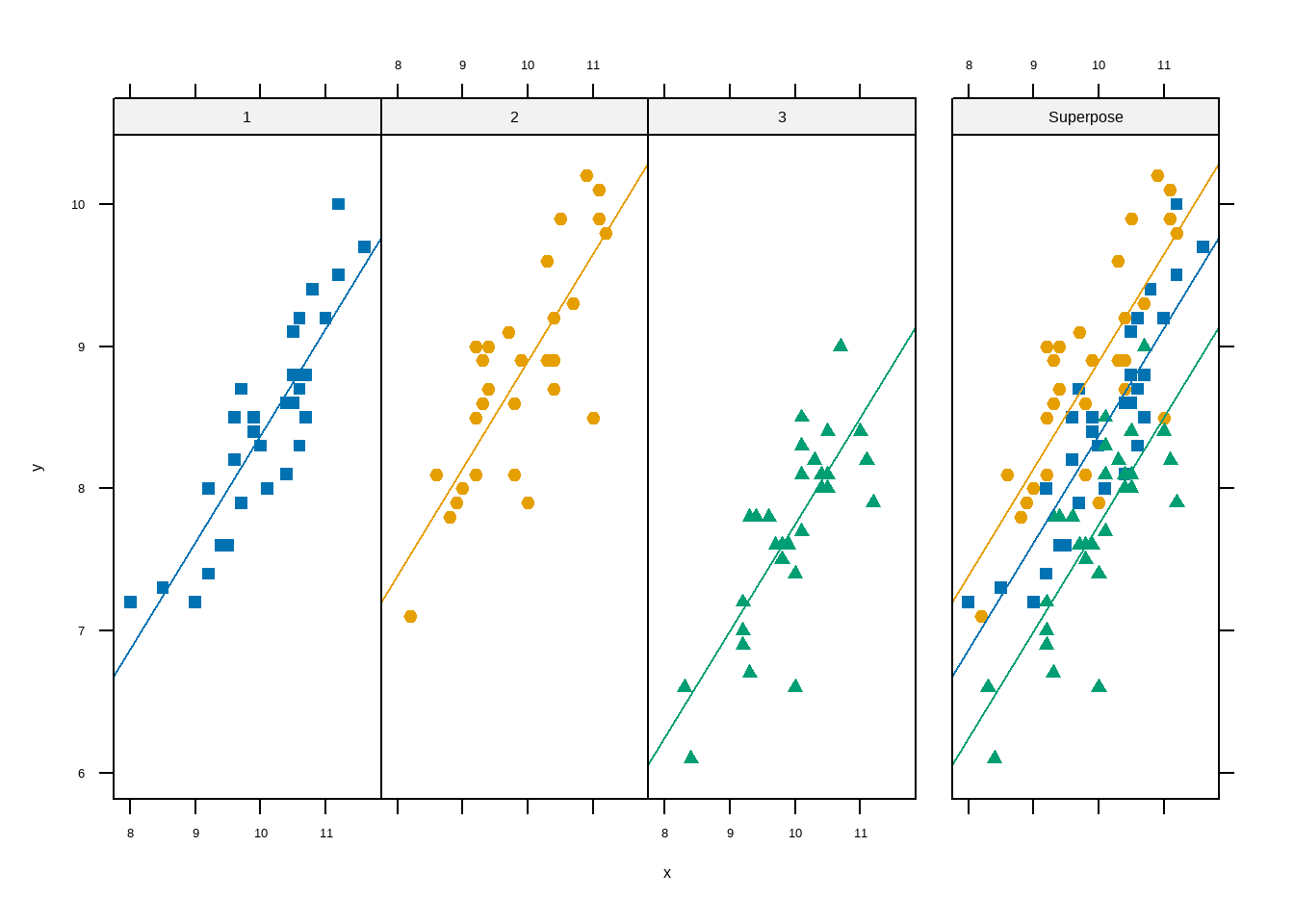
但其实我们也可以用ggplot2来画,可能更好看一点:
theme_set(theme_bw())

p1 <- ggplot(df13_11, aes(x=x,y=y))+
  geom_point(aes(color=group,shape=group))+
  geom_smooth(method = "lm",se=F,aes(color=group))+
  labs(y=NULL)

p2 <- ggplot(df13_11, aes(x=x,y=y))+
  geom_point(aes(color=group,shape=group))+
  geom_smooth(method = "lm",se=F,aes(color=group))+
  facet_wrap(~group)

library(patchwork)
p2 + p1 + plot_layout(guides = 'collect',widths = c(3, 1))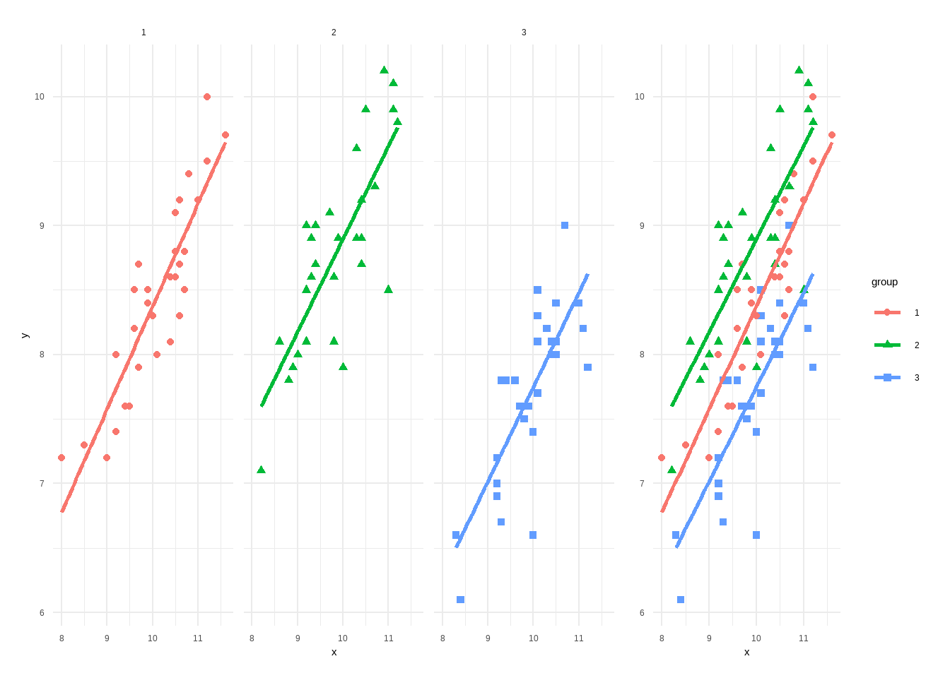
好看是好看,但是很明显不如HH简洁啊!
17.2 使用rstatix进行优雅的协方差分析
library(rstatix)

res <- anova_test(y ~ x + group, data = df13_11, type = 1)#不同类型可选
get_anova_table(res)
## ANOVA Table (type I tests)
##
##   Effect DFn DFd       F        p p<.05   ges
## 1      x   1  86 171.199 3.64e-22     * 0.666
## 2  group   2  86  58.480 9.22e-17     * 0.576
结果也是一样的!
17.3 随机区组设计资料的协方差分析
使用课本例13-2的数据。
df <- foreign::read.spss("datasets/例13-02.sav",to.data.frame = T,
                         reencode = "utf-8")
df$block <- factor(df$block)

str(df)
## 'data.frame':    36 obs. of  4 variables:
##  $ x    : num  257 272 210 300 262 ...
##  $ y    : num  27 41.7 25 52 14.5 48.8 48 9.5 37 56.5 ...
##  $ group: Factor w/ 3 levels "A....","B....",..: 1 1 1 1 1 1 1 1 1 1 ...
##  $ block: Factor w/ 12 levels "1","2","3","4",..: 1 2 3 4 5 6 7 8 9 10 ...
##  - attr(*, "variable.labels")= Named chr [1:4] "..ʳ.." ".........." "........" "......"
##   ..- attr(*, "names")= chr [1:4] "x" "y" "group" "block"
head(df)
##       x    y group block
## 1 256.9 27.0 A....     1
## 2 271.6 41.7 A....     2
## 3 210.2 25.0 A....     3
## 4 300.1 52.0 A....     4
## 5 262.2 14.5 A....     5
## 6 304.4 48.8 A....     6
进行随机区组设计的协方差分析:
fit <- aov(y ~ x + block + group, data = df) # 注意顺序
summary(fit)
##             Df Sum Sq Mean Sq F value  Pr(>F)
## x            1  69073   69073 651.823 < 2e-16 ***
## block       11   4024     366   3.452 0.00711 **
## group        2    464     232   2.189 0.13692
## Residuals   21   2225     106
## ---
## Signif. codes:  0 '***' 0.001 '**' 0.01 '*' 0.05 '.' 0.1 ' ' 1

car::Anova(fit)
## Anova Table (Type II tests)
##
## Response: y
##           Sum Sq Df F value    Pr(>F)
## x         6174.2  1 58.2643 1.733e-07 ***
## block     3765.3 11  3.2302   0.01009 *
## group      463.9  2  2.1891   0.13692
## Residuals 2225.4 21
## ---
## Signif. codes:  0 '***' 0.001 '**' 0.01 '*' 0.05 '.' 0.1 ' ' 1
结果和课本一致。
或者用rstatix:
fit <- anova_test(y ~ x + block + group, data = df, type = 3)
get_anova_table(fit)
## ANOVA Table (type III tests)
##
##   Effect DFn DFd      F        p p<.05   ges
## 1      x   1  21 58.264 1.73e-07     * 0.735
## 2  block  11  21  3.230 1.00e-02     * 0.629
## 3  group   2  21  2.189 1.37e-01       0.173