library(compareGroups)
data("regicor")
dim(regicor)
## [1] 2294   25
str(regicor)
## 'data.frame':    2294 obs. of  25 variables:
##  $ id      : num  2.26e+03 1.88e+03 3.00e+09 3.00e+09 3.00e+09 ...
##   ..- attr(*, "label")= Named chr "Individual id"
##   .. ..- attr(*, "names")= chr "id"
##  $ year    : Factor w/ 3 levels "1995","2000",..: 3 3 2 2 2 2 2 1 3 1 ...
##   ..- attr(*, "label")= Named chr "Recruitment year"
##   .. ..- attr(*, "names")= chr "year"
##  $ age     : int  70 56 37 69 70 40 66 53 43 70 ...
##   ..- attr(*, "label")= Named chr "Age"
##   .. ..- attr(*, "names")= chr "age"
##  $ sex     : Factor w/ 2 levels "Male","Female": 2 2 1 2 2 2 1 2 2 1 ...
##   ..- attr(*, "label")= chr "Sex"
##  $ smoker  : Factor w/ 3 levels "Never smoker",..: 1 1 2 1 NA 2 1 1 3 3 ...
##   ..- attr(*, "label")= Named chr "Smoking status"
##   .. ..- attr(*, "names")= chr "smoker"
##  $ sbp     : int  138 139 132 168 NA 108 120 132 95 142 ...
##   ..- attr(*, "label")= Named chr "Systolic blood pressure"
##   .. ..- attr(*, "names")= chr "sbp"
##  $ dbp     : int  75 89 82 97 NA 70 72 78 65 78 ...
##   ..- attr(*, "label")= Named chr "Diastolic blood pressure"
##   .. ..- attr(*, "names")= chr "dbp"
##  $ histhtn : Factor w/ 2 levels "Yes","No": 2 2 2 2 2 2 1 2 2 2 ...
##   ..- attr(*, "label")= Named chr "History of hypertension"
##   .. ..- attr(*, "names")= chr "histbp"
##  $ txhtn   : Factor w/ 2 levels "No","Yes": 1 1 1 1 1 1 2 1 1 1 ...
##   ..- attr(*, "label")= chr "Hypertension treatment"
##  $ chol    : num  294 220 245 168 NA NA 298 254 194 188 ...
##   ..- attr(*, "label")= Named chr "Total cholesterol"
##   .. ..- attr(*, "names")= chr "chol"
##  $ hdl     : num  57 50 59.8 53.2 NA ...
##   ..- attr(*, "label")= Named chr "HDL cholesterol"
##   .. ..- attr(*, "names")= chr "hdl"
##  $ triglyc : num  93 160 89 116 NA 94 71 NA 68 137 ...
##   ..- attr(*, "label")= Named chr "Triglycerides"
##   .. ..- attr(*, "names")= chr "triglyc"
##  $ ldl     : num  218.4 138 167.4 91.6 NA ...
##   ..- attr(*, "label")= Named chr "LDL cholesterol"
##   .. ..- attr(*, "names")= chr "ldl"
##  $ histchol: Factor w/ 2 levels "Yes","No": 2 2 2 2 NA 2 1 2 2 2 ...
##   ..- attr(*, "label")= chr "History of hyperchol."
##  $ txchol  : Factor w/ 2 levels "No","Yes": 1 1 1 1 NA 1 1 1 1 1 ...
##   ..- attr(*, "label")= Named chr "Cholesterol treatment"
##   .. ..- attr(*, "names")= chr "txchol"
##  $ height  : num  160 163 170 147 NA ...
##   ..- attr(*, "label")= Named chr "Height (cm)"
##   .. ..- attr(*, "names")= chr "height"
##  $ weight  : num  64 67 70 68 NA 43.5 79.2 45.8 53 62 ...
##   ..- attr(*, "label")= Named chr "Weight (Kg)"
##   .. ..- attr(*, "names")= chr "weight"
##  $ bmi     : num  25 25.2 24.2 31.5 NA ...
##   ..- attr(*, "label")= Named chr "Body mass index"
##   .. ..- attr(*, "names")= chr "bmi"
##  $ phyact  : num  304 160 553 522 NA ...
##   ..- attr(*, "label")= Named chr "Physical activity (Kcal/week)"
##   .. ..- attr(*, "names")= chr "phyact"
##  $ pcs     : num  54.5 58.2 43.4 54.3 NA ...
##   ..- attr(*, "label")= Named chr "Physical component"
##   .. ..- attr(*, "names")= chr "pcs"
##  $ mcs     : num  58.9 48 62.6 57.9 NA ...
##   ..- attr(*, "label")= chr "Mental component"
##  $ cv      : Factor w/ 2 levels "No","Yes": 1 1 1 1 NA 1 1 1 1 1 ...
##   ..- attr(*, "label")= chr "Cardiovascular event"
##  $ tocv    : num  1025 2757 1906 1055 NA ...
##   ..- attr(*, "label")= chr "Days to cardiovascular event or end of follow-up"
##  $ death   : Factor w/ 2 levels "No","Yes": 2 1 1 1 NA 1 2 1 1 1 ...
##   ..- attr(*, "label")= chr "Overall death"
##  $ todeath : num  1299.2 39.3 858.4 1833.1 NA ...
## ..- attr(*, "label")= chr "Days to overall death or end of follow-up"7 三线表和统计绘图
本章对应课本中的第十章,统计表主要是三线表的绘制,其实这是Word的功能,R语言中的三线表绘制绘制R包通常都是用于绘制各类SCI文献中的第一张表,比如各种基线资料表、人口统计学资料表等。
统计绘图则是介绍各种常用的统计图形,比如:条形图、箱线图、直方图、饼图、茎叶图、地图等。
7.1 统计表
主要是各种三线表的绘制,但是目前的临床研究的三线表制作还是离不开Word、Excel等传统软件,目前没有任何一款R包可以做到:输出结果无需修改即可直接发表。或多或少都需要在Word中修改一下的。
目前在R语言中绘制三线表的常见R包有:compareGroups、tableone、table1、gtSummary、gt、gtExtras等,我已写过多篇推文进行介绍(公众号后台回复三线表即可获取合集):
compareGroups:compareGroups包1行代码生成基线资料表tableone:使用R语言快速绘制三线表table1:tableone?table1?傻傻分不清楚gtSummary:超棒的三线表绘制工具,总有一款适合你gt:gt包绘制表格详细介绍gtExtras:使用gtExtras美化表格
我使用下来在多数情况下还是compareGroups最方便,所以下面将会详细介绍compareGroups的用法,其他R包的用法请参考以上链接。
7.1.1 compareGroups
compareGroups可用一句代码生成基线资料表、单因素分析表、多因素分析表等,可直接把结果导出为csv、Excel、Word、Markdown、LaTeX、PDF,而且十分美观,大大提高工作效率。
之前也做过介绍,但是最近发现R包更新后自带数据换了,之前的predimed数据没有了,变成了regicor,所以重新再整理一遍。之前的介绍:使用compareGroups包1行代码生成基线资料表
官方文档的名字就叫:分组描述(Descriptives-by-groups),充分说明该包的强项就是分组描述,特别适合基线资料表、各类SCI中的table 1的绘制。支持生存数据,可以计算HR、OR、P-for-trend、多重检验的P值等。
使用方法和之前介绍的基本一样,主要就是3个函数:
compareGroups:计算createTable:构建表格export2xxx导出表格
之前R包内置的predimed已经没有了,现在默认演示数据变成了regicor。
为了说明这个软件包是如何工作的,我们从REGICOR研究中取了一部分数据。REGICOR是一个 对来自西班牙东北部的参与者进行的横断面研究,包括:人口统计学信息(年龄、性别、身高、体重、腰围等)、血脂特征(总胆固醇和胆固醇、甘油三酯等)、问卷调查信息(体格,活动,生活质量,…)等。此外,心血管事件和 死亡信息来自医院和官方登记处。
查看数据:
各个变量的信息如下:
| Name | Label | Codes |
|---|---|---|
| id | Individual id | |
| year | Recruitment year | 1995; 2000; 2005 |
| age | Age | |
| sex | Sex | Male; Female |
| smoker | Smoking status | Never smoker; Current or former < 1y; Former $\geq$ 1y |
| sbp | Systolic blood pressure | |
| dbp | Diastolic blood pressure | |
| histhtn | History of hypertension | Yes; No |
| txhtn | Hypertension treatment | No; Yes |
| chol | Total cholesterol | |
| hdl | HDL cholesterol | |
| triglyc | Triglycerides | |
| ldl | LDL cholesterol | |
| histchol | History of hyperchol. | Yes; No |
| txchol | Cholesterol treatment | No; Yes |
| height | Height (cm) | |
| weight | Weight (Kg) | |
| bmi | Body mass index | |
| phyact | Physical activity (Kcal/week) | |
| pcs | Physical component | |
| mcs | Mental component | |
| cv | Cardiovascular event | No; Yes |
| tocv | Days to cardiovascular event or end of follow-up | |
| death | Overall death | No; Yes |
| todeath | Days to overall death or end of follow-up |
使用该R包的一些注意点:
- 该包的重点是描述数据,不是对数据进行质量控制或其他目的。
- 强烈建议数据框中只包含需要描述的数据,对于不需要的数据建议不要包含在数据框中。
- 分类变量需要进行因子化。
- 可以给各个变量增加
label属性以展示其详细信息,该包默认会展示各个变量的label。
如果是生存数据(time-to-event),必须使用Surv()包装数据。比如:
library(survival)

regicor$tmain <- with(regicor, Surv(tocv, cv == "Yes"))
attr(regicor$tmain, "label") <- "Time to CV event or censoring"这里新建的tmain是生存时间。
以year为分组变量,统计各个变量的差异:
# 不要id这个变量
compareGroups(year ~ . - id, data=regicor)
##
##
## -------- Summary of results by groups of 'Recruitment year'---------
##
##
##    var                                              N    p.value
## 1  Age                                              2294 0.078*
## 2  Sex                                              2294 0.506
## 3  Smoking status                                   2233 <0.001**
## 4  Systolic blood pressure                          2280 <0.001**
## 5  Diastolic blood pressure                         2280 <0.001**
## 6  History of hypertension                          2286 <0.001**
## 7  Hypertension treatment                           2251 0.002**
## 8  Total cholesterol                                2193 <0.001**
## 9  HDL cholesterol                                  2225 0.208
## 10 Triglycerides                                    2231 0.582
## 11 LDL cholesterol                                  2126 <0.001**
## 12 History of hyperchol.                            2273 <0.001**
## 13 Cholesterol treatment                            2239 <0.001**
## 14 Height (cm)                                      2259 0.003**
## 15 Weight (Kg)                                      2259 0.150
## 16 Body mass index                                  2259 <0.001**
## 17 Physical activity (Kcal/week)                    2206 <0.001**
## 18 Physical component                               2054 0.032**
## 19 Mental component                                 2054 <0.001**
## 20 Cardiovascular event                             2163 0.161
## 21 Days to cardiovascular event or end of follow-up 2163 0.099*
## 22 Overall death                                    2148 <0.001**
## 23 Days to overall death or end of follow-up        2148 0.252
## 24 Time to CV event or censoring                    2163 0.157
##    method            selection
## 1  continuous normal ALL
## 2  categorical       ALL
## 3  categorical       ALL
## 4  continuous normal ALL
## 5  continuous normal ALL
## 6  categorical       ALL
## 7  categorical       ALL
## 8  continuous normal ALL
## 9  continuous normal ALL
## 10 continuous normal ALL
## 11 continuous normal ALL
## 12 categorical       ALL
## 13 categorical       ALL
## 14 continuous normal ALL
## 15 continuous normal ALL
## 16 continuous normal ALL
## 17 continuous normal ALL
## 18 continuous normal ALL
## 19 continuous normal ALL
## 20 categorical       ALL
## 21 continuous normal ALL
## 22 categorical       ALL
## 23 continuous normal ALL
## 24 Surv [Tmax=1718]  ALL
## -----
## Signif. codes: 0 '**' 0.05 '*' 0.1 ' ' 1比如第一个变量age,其实使用的方差分析,给出了age在不同year中的pvalue,method显示了该包把age这个变量看做连续型变量且符合正态分布。
我们可以自己使用方差分析看下结果:
summary(aov(age ~ year, data = regicor))
##               Df Sum Sq Mean Sq F value Pr(>F)
## year           2    623   311.6   2.556 0.0778 .
## Residuals   2291 279320   121.9
## ---
## Signif. codes:  0 '***' 0.001 '**' 0.01 '*' 0.05 '.' 0.1 ' ' 1
可以看到结果是一样的哈~
sex这个变量是用的卡方检验:
chisq.test(regicor$sex, regicor$year)
##
##  Pearson's Chi-squared test
##
## data:  regicor$sex and regicor$year
## X-squared = 1.364, df = 2, p-value = 0.5056
结果也是一样的。
支持之使用其中一部分数据,比如只看一下age、smoker、bmi这3个变量在不同的year中的差异,并且只选择性别为女性,对于bmi这个变量,只选择年龄大于50岁的:
compareGroups(year ~ age + smoker + bmi, data=regicor,
              selec = list(bmi=age>50),
              subset = sex=="Female")
##
##
## -------- Summary of results by groups of 'year'---------
##
##
##   var             N    p.value  method
## 1 Age             1193 0.351    continuous normal
## 2 Smoking status  1162 <0.001** categorical
## 3 Body mass index  709 0.308    continuous normal
##   selection
## 1 sex == "Female"
## 2 sex == "Female"
## 3 (sex == "Female") & (age > 50)
## -----
## Signif. codes: 0 '**' 0.05 '*' 0.1 ' ' 1连续型变量支持选择不同的统计方法(选择有限),通过method指定即可:
compareGroups(year ~ age + smoker + triglyc, data=regicor,
              method = c(triglyc=NA),
              alpha= 0.01)
## Warning in cor.test.default(x, as.integer(y), method = "spearman"): Cannot
## compute exact p-value with ties
##
##
## -------- Summary of results by groups of 'Recruitment year'---------
##
##
##   var            N    p.value  method                selection
## 1 Age            2294 0.078*   continuous normal     ALL
## 2 Smoking status 2233 <0.001** categorical           ALL
## 3 Triglycerides  2231 0.762    continuous non-normal ALL
## -----
## Signif. codes: 0 '**' 0.05 '*' 0.1 ' ' 1method:统计检验方法- 1:数值型变量,正态分布,
- 2:数值型变量,非正态分布
- 3:分类变量
- NA:使用
shapiro.test()决定是否正态分布
alpha:正态性检验的阈值min.dis:所有非因子型向量都会被认为是连续型的,除非某个变量的取值少于5个,可通过此参数更改这个标准。
regicor$age7gr <- as.integer(cut(regicor$age, breaks = c(-Inf, 40, 45, 50, 55, 65, 70, Inf), right = TRUE))

compareGroups(year ~ age7gr, data = regicor, method = c(age7gr = NA), min.dis = 8)
## Warning in compare.i(X[, i], y = y, selec.i = selec[i], method.i = method[i], :
## variable 'age7gr' converted to factor since few different values contained
##
##
## -------- Summary of results by groups of 'Recruitment year'---------
##
##
##   var    N    p.value method      selection
## 1 age7gr 2294 0.012** categorical ALL
## -----
## Signif. codes: 0 '**' 0.05 '*' 0.1 ' ' 1max.ylev:分组变量的最大组数
compareGroups(age7gr ~ sex + bmi + smoker, data = regicor, max.ylev = 7)
##
##
## -------- Summary of results by groups of 'age7gr'---------
##
##
##   var             N    p.value  method            selection
## 1 Sex             2294 0.950    categorical       ALL
## 2 Body mass index 2259 <0.001** continuous normal ALL
## 3 Smoking status  2233 <0.001** categorical       ALL
## -----
## Signif. codes: 0 '**' 0.05 '*' 0.1 ' ' 1显示列的名字,而不是label:
compareGroups(year ~ age + smoker + bmi, data = regicor, include.label = FALSE)
##
##
## -------- Summary of results by groups of 'year'---------
##
##
##   var    N    p.value  method            selection
## 1 age    2294 0.078*   continuous normal ALL
## 2 smoker 2233 <0.001** categorical       ALL
## 3 bmi    2259 <0.001** continuous normal ALL
## -----
## Signif. codes: 0 '**' 0.05 '*' 0.1 ' ' 1Q1/Q3:非正态分布的变量默认显示中位数(25%,75%),这个百分位数可以更改,设置为0和1则是最小值和最大值
resu2 <- compareGroups(year ~ age + triglyc, data = regicor,
                       method = c(triglyc = 2),
                       Q1 = 0.025, Q3 = 0.975)
## Warning in cor.test.default(x, as.integer(y), method = "spearman"): Cannot
## compute exact p-value with ties
createTable(resu2)
##
## --------Summary descriptives table by 'Recruitment year'---------
##
## _______________________________________________________________________
##                    1995            2000            2005       p.overall
##                    N=431           N=786          N=1077
## ¯¯¯¯¯¯¯¯¯¯¯¯¯¯¯¯¯¯¯¯¯¯¯¯¯¯¯¯¯¯¯¯¯¯¯¯¯¯¯¯¯¯¯¯¯¯¯¯¯¯¯¯¯¯¯¯¯¯¯¯¯¯¯¯¯¯¯¯¯¯¯
## Age             54.1 (11.7)     54.3 (11.2)     55.3 (10.6)     0.078
## Triglycerides 94.0 [47.0;292] 98.0 [47.0;278] 98.0 [42.0;293]   0.762
## ¯¯¯¯¯¯¯¯¯¯¯¯¯¯¯¯¯¯¯¯¯¯¯¯¯¯¯¯¯¯¯¯¯¯¯¯¯¯¯¯¯¯¯¯¯¯¯¯¯¯¯¯¯¯¯¯¯¯¯¯¯¯¯¯¯¯¯¯¯¯¯simplify:有时某个变量在某个分组中可能样本数为0,这时候要设置为TRUE来排除这样的亚组,因为卡方检验和Fisher精确概率法的计算不能为0。
下面新建一个变量smk,其中unknown这个分组的样本数为0:
regicor$smk <- regicor$smoker
levels(regicor$smk) <- c("Never smoker", "Current or former < 1y", "Former >= 1y", "Unknown")
attr(regicor$smk, "label") <- "Smoking 4 cat."
cbind(table(regicor$smk))
##                        [,1]
## Never smoker           1201
## Current or former < 1y  593
## Former >= 1y            439
## Unknown 0如果不加simplify = FALSE会给出warning:
compareGroups(year ~ age + smk + bmi, data = regicor)
## Warning in compare.i(X[, i], y = y, selec.i = selec[i], method.i = method[i], :
## Some levels of 'smk' are removed since no observation in that/those levels
##
##
## -------- Summary of results by groups of 'Recruitment year'---------
##
##
##   var             N    p.value  method            selection
## 1 Age             2294 0.078*   continuous normal ALL
## 2 Smoking 4 cat.  2233 <0.001** categorical       ALL
## 3 Body mass index 2259 <0.001** continuous normal ALL
## -----
## Signif. codes: 0 '**' 0.05 '*' 0.1 ' ' 1加simplify = FALSE之后就不再对这个变量进行统计检验了,也就没有P值显示了:
compareGroups(year ~ age + smk + bmi, data = regicor, simplify = FALSE)
##
##
## -------- Summary of results by groups of 'Recruitment year'---------
##
##
##   var             N    p.value  method            selection
## 1 Age             2294 0.078*   continuous normal ALL
## 2 Smoking 4 cat.  2233 .        categorical       ALL
## 3 Body mass index 2259 <0.001** continuous normal ALL
## -----
## Signif. codes:  0 '**' 0.05 '*' 0.1 ' ' 1
支持更新对象:
res <- compareGroups(year ~ age + sex + smoker + bmi, data = regicor)
res
##
##
## -------- Summary of results by groups of 'Recruitment year'---------
##
##
##   var             N    p.value  method            selection
## 1 Age             2294 0.078*   continuous normal ALL
## 2 Sex             2294 0.506    categorical       ALL
## 3 Smoking status  2233 <0.001** categorical       ALL
## 4 Body mass index 2259 <0.001** continuous normal ALL
## -----
## Signif. codes:  0 '**' 0.05 '*' 0.1 ' ' 1
res <- update(res, . ~ . - sex + triglyc + cv + tocv,
subset = sex == "Female",
method = c(triglyc = 2, tocv = 2),
selec = list(triglyc = txchol == "No"))
## Warning in cor.test.default(x, as.integer(y), method = "spearman"): Cannot
## compute exact p-value with ties
## Warning in cor.test.default(x, as.integer(y), method = "spearman"): Cannot
## compute exact p-value with ties
res
##
##
## -------- Summary of results by groups of 'year'---------
##
##
## var N p.value
## 1 Age 1193 0.351
## 2 Smoking status 1162 <0.001**
## 3 Body mass index 1169 0.084*
## 4 Triglycerides 1020 0.993
## 5 Cardiovascular event 1121 0.139
## 6 Days to cardiovascular event or end of follow-up 1121 0.427
## method selection
## 1 continuous normal sex == "Female"
## 2 categorical sex == "Female"
## 3 continuous normal sex == "Female"
## 4 continuous non-normal (sex == "Female") & (txchol == "No")
## 5 categorical sex == "Female"
## 6 continuous non-normal sex == "Female"
## -----
## Signif. codes: 0 '**' 0.05 '*' 0.1 ' ' 1支持提取其中的某些信息,比如P值、均值等,方便后续的操作:
data(SNPs)
tab <- createTable(compareGroups(casco ~ snp10001 + snp10002 + snp10005 +
                                   snp10008 + snp10009, SNPs))
## Warning in chisq.test(xx, correct = FALSE): Chi-squared approximation may be
## incorrect
## Warning in chisq.test(xx, correct = FALSE): Chi-squared approximation may be
## incorrect
## Warning in chisq.test(xx, correct = FALSE): Chi-squared approximation may be
## incorrect

# 提取P值,方便进行校正
pvals <- getResults(tab, "p.overall")
p.adjust(pvals, method = "BH")
##  snp10001  snp10002  snp10005  snp10008  snp10009
## 0.7051300 0.7072158 0.7583432 0.7583432 0.70721584.6.0以后的版本还增加了计算调整P值的方法,和p.adjust的方法一样,比如Bonferroni/False Discovery Rate等。
cg <- compareGroups(casco ~ snp10001 + snp10002 + snp10005 + snp10008 + snp10009, SNPs)
## Warning in chisq.test(xx, correct = FALSE): Chi-squared approximation may be
## incorrect
## Warning in chisq.test(xx, correct = FALSE): Chi-squared approximation may be
## incorrect
## Warning in chisq.test(xx, correct = FALSE): Chi-squared approximation may be
## incorrect
createTable(padjustCompareGroups(cg, method = "BH"))
##
## --------Summary descriptives table by 'casco'---------
##
## _________________________________________
##               0          1      p.overall
##              N=47      N=110
## ¯¯¯¯¯¯¯¯¯¯¯¯¯¯¯¯¯¯¯¯¯¯¯¯¯¯¯¯¯¯¯¯¯¯¯¯¯¯¯¯¯
## snp10001:                         0.705
##     CC    2 (4.26%)  10 (9.09%)
##     CT    21 (44.7%) 32 (29.1%)
##     TT    24 (51.1%) 68 (61.8%)
## snp10002:                         0.707
##     AA    0 (0.00%)  5 (4.55%)
##     AC    25 (53.2%) 53 (48.2%)
##     CC    22 (46.8%) 52 (47.3%)
## snp10005:                         0.758
##     AA    0 (0.00%)  3 (2.73%)
##     AG    22 (46.8%) 48 (43.6%)
##     GG    25 (53.2%) 59 (53.6%)
## snp10008:                         0.758
##     CC    30 (63.8%) 74 (67.3%)
##     CG    15 (31.9%) 29 (26.4%)
##     GG    2 (4.26%)  7 (6.36%)
## snp10009:                         0.707
##     AA    21 (45.7%) 51 (46.4%)
##     AG    25 (54.3%) 54 (49.1%)
##     GG    0 (0.00%)  5 (4.55%)
## ¯¯¯¯¯¯¯¯¯¯¯¯¯¯¯¯¯¯¯¯¯¯¯¯¯¯¯¯¯¯¯¯¯¯¯¯¯¯¯¯¯
支持计算OR值和HR值,如果是二分类会计算OR值,如果是time-to-event数据会计算HR值:
# show.ratio = TRUE展示p.ratio和OR值
res1 <- compareGroups(cv ~ age + sex + bmi + smoker, data = regicor, ref = 1)
createTable(res1, show.ratio = TRUE)
##
## --------Summary descriptives table by 'Cardiovascular event'---------
##
## ______________________________________________________________________________________
##                                 No          Yes            OR        p.ratio p.overall
##                               N=2071       N=92
## ¯¯¯¯¯¯¯¯¯¯¯¯¯¯¯¯¯¯¯¯¯¯¯¯¯¯¯¯¯¯¯¯¯¯¯¯¯¯¯¯¯¯¯¯¯¯¯¯¯¯¯¯¯¯¯¯¯¯¯¯¯¯¯¯¯¯¯¯¯¯¯¯¯¯¯¯¯¯¯¯¯¯¯¯¯¯
## Age                        54.6 (11.1)  57.5 (11.0) 1.02 [1.00;1.04]  0.017    0.018
## Sex:                                                                           0.801
##     Male                   996 (48.1%)  46 (50.0%)        Ref.        Ref.
##     Female                 1075 (51.9%) 46 (50.0%)  0.93 [0.61;1.41]  0.721
## Body mass index            27.6 (4.56)  28.1 (4.48) 1.02 [0.98;1.07]  0.313    0.307
## Smoking status:                                                               <0.001
##     Never smoker           1099 (54.3%) 37 (40.2%)        Ref.        Ref.
##     Current or former < 1y 506 (25.0%)  47 (51.1%)  2.75 [1.77;4.32] <0.001
##     Former >= 1y           419 (20.7%)   8 (8.70%)  0.58 [0.25;1.19]  0.142
## ¯¯¯¯¯¯¯¯¯¯¯¯¯¯¯¯¯¯¯¯¯¯¯¯¯¯¯¯¯¯¯¯¯¯¯¯¯¯¯¯¯¯¯¯¯¯¯¯¯¯¯¯¯¯¯¯¯¯¯¯¯¯¯¯¯¯¯¯¯¯¯¯¯¯¯¯¯¯¯¯¯¯¯¯¯¯ref可以更改参考水平,比如smoker以第一个水平为参考,sex以第二个水平为参考:
res2 <- compareGroups(cv ~ age + sex + bmi + smoker, data = regicor,
                      ref = c(smoker = 1, sex = 2))
createTable(res2, show.ratio = TRUE)
##
## --------Summary descriptives table by 'Cardiovascular event'---------
##
## ______________________________________________________________________________________
##                                 No          Yes            OR        p.ratio p.overall
##                               N=2071       N=92
## ¯¯¯¯¯¯¯¯¯¯¯¯¯¯¯¯¯¯¯¯¯¯¯¯¯¯¯¯¯¯¯¯¯¯¯¯¯¯¯¯¯¯¯¯¯¯¯¯¯¯¯¯¯¯¯¯¯¯¯¯¯¯¯¯¯¯¯¯¯¯¯¯¯¯¯¯¯¯¯¯¯¯¯¯¯¯
## Age                        54.6 (11.1)  57.5 (11.0) 1.02 [1.00;1.04]  0.017    0.018
## Sex:                                                                           0.801
##     Male                   996 (48.1%)  46 (50.0%)  1.08 [0.71;1.64]  0.721
##     Female                 1075 (51.9%) 46 (50.0%)        Ref.        Ref.
## Body mass index            27.6 (4.56)  28.1 (4.48) 1.02 [0.98;1.07]  0.313    0.307
## Smoking status:                                                               <0.001
##     Never smoker           1099 (54.3%) 37 (40.2%)        Ref.        Ref.
##     Current or former < 1y 506 (25.0%)  47 (51.1%)  2.75 [1.77;4.32] <0.001
##     Former >= 1y           419 (20.7%)   8 (8.70%)  0.58 [0.25;1.19]  0.142
## ¯¯¯¯¯¯¯¯¯¯¯¯¯¯¯¯¯¯¯¯¯¯¯¯¯¯¯¯¯¯¯¯¯¯¯¯¯¯¯¯¯¯¯¯¯¯¯¯¯¯¯¯¯¯¯¯¯¯¯¯¯¯¯¯¯¯¯¯¯¯¯¯¯¯¯¯¯¯¯¯¯¯¯¯¯¯这里的p.overall是通过t检验计算的:(如果不符合正态分布是通过Kruskall-Wallis检验计算)
t.test(age ~ cv, data = regicor)
##
##  Welch Two Sample t-test
##
## data:  age by cv
## t = -2.4124, df = 99.303, p-value = 0.01768
## alternative hypothesis: true difference in means between group No and group Yes is not equal to 0
## 95 percent confidence interval:
##  -5.1660205 -0.5031794
## sample estimates:
##  mean in group No mean in group Yes
## 54.62192 57.45652这个表格中的p.ratio和OR值就是做个逻辑回归得到的:
aa <- glm(cv ~ age, data = regicor,family = binomial())
broom::tidy(aa,exponentiate = T,conf.int = T)
## # A tibble: 2 × 7
##   term        estimate std.error statistic  p.value conf.low conf.high
##   <chr>          <dbl>     <dbl>     <dbl>    <dbl>    <dbl>     <dbl>
## 1 (Intercept)   0.0120   0.572       -7.74 1.01e-14  0.00377    0.0357
## 2 age 1.02 0.00980 2.39 1.69e- 2 1.00 1.04age的p.value就是表格中的p.ratio,estimate是OR值,conf.low和conf.high是可信区间。
ref.no表示,如果某个变量中有No(或者NO,no,不区分大小写)这个类别,那就以这个类别为参考,这是一个可适用于所有变量的参数。
res <- compareGroups(cv ~ age + sex + bmi + histhtn + txhtn, data = regicor,
                     ref.no = "NO")
createTable(res, show.ratio = TRUE)
##
## --------Summary descriptives table by 'Cardiovascular event'---------
##
## ____________________________________________________________________________________
##                               No          Yes            OR        p.ratio p.overall
##                             N=2071       N=92
## ¯¯¯¯¯¯¯¯¯¯¯¯¯¯¯¯¯¯¯¯¯¯¯¯¯¯¯¯¯¯¯¯¯¯¯¯¯¯¯¯¯¯¯¯¯¯¯¯¯¯¯¯¯¯¯¯¯¯¯¯¯¯¯¯¯¯¯¯¯¯¯¯¯¯¯¯¯¯¯¯¯¯¯¯
## Age                      54.6 (11.1)  57.5 (11.0) 1.02 [1.00;1.04]  0.017    0.018
## Sex:                                                                         0.801
##     Male                 996 (48.1%)  46 (50.0%)        Ref.        Ref.
##     Female               1075 (51.9%) 46 (50.0%)  0.93 [0.61;1.41]  0.721
## Body mass index          27.6 (4.56)  28.1 (4.48) 1.02 [0.98;1.07]  0.313    0.307
## History of hypertension:                                                     0.058
##     Yes                  647 (31.3%)  38 (41.3%)  1.54 [1.00;2.36]  0.049
##     No                   1418 (68.7%) 54 (58.7%)        Ref.        Ref.
## Hypertension treatment:                                                      0.270
##     No                   1657 (81.3%) 70 (76.1%)        Ref.        Ref.
##     Yes                  382 (18.7%)  22 (23.9%)  1.37 [0.82;2.21]  0.223
## ¯¯¯¯¯¯¯¯¯¯¯¯¯¯¯¯¯¯¯¯¯¯¯¯¯¯¯¯¯¯¯¯¯¯¯¯¯¯¯¯¯¯¯¯¯¯¯¯¯¯¯¯¯¯¯¯¯¯¯¯¯¯¯¯¯¯¯¯¯¯¯¯¯¯¯¯¯¯¯¯¯¯¯¯sex/histhtn/txhtn这几个变量中都有No这个分类,所以都以这个类别为参考。
对于连续性变量来说,OR值和HR值的解释是自变量每增加一个单位,因变量变化OR倍或HR倍,参数fact.ratio可以控制一个单位具体是多少。比如设置bmi的一个单位是2,age的一个单位是10:
res <- compareGroups(cv ~ age + bmi, data = regicor,
                     fact.ratio = c(age = 10, bmi = 2))
createTable(res, show.ratio = TRUE)
##
## --------Summary descriptives table by 'Cardiovascular event'---------
##
## __________________________________________________________________________
##                     No          Yes            OR        p.ratio p.overall
##                   N=2071       N=92
## ¯¯¯¯¯¯¯¯¯¯¯¯¯¯¯¯¯¯¯¯¯¯¯¯¯¯¯¯¯¯¯¯¯¯¯¯¯¯¯¯¯¯¯¯¯¯¯¯¯¯¯¯¯¯¯¯¯¯¯¯¯¯¯¯¯¯¯¯¯¯¯¯¯¯
## Age             54.6 (11.1) 57.5 (11.0) 1.26 [1.04;1.53]  0.017    0.018
## Body mass index 27.6 (4.56) 28.1 (4.48) 1.05 [0.96;1.14]  0.313    0.307
## ¯¯¯¯¯¯¯¯¯¯¯¯¯¯¯¯¯¯¯¯¯¯¯¯¯¯¯¯¯¯¯¯¯¯¯¯¯¯¯¯¯¯¯¯¯¯¯¯¯¯¯¯¯¯¯¯¯¯¯¯¯¯¯¯¯¯¯¯¯¯¯¯¯¯通常对于OR值和HR值来说,是相对于因变量的某个类别来说的,比如自变量每增加一个单位,患癌症的风险增加OR倍,可以通过ref.y改成不患癌症的风险增加xx倍。
res <- compareGroups(cv ~ age + sex + bmi + txhtn, data = regicor, ref.y = 2)
createTable(res, show.ratio = TRUE)
##
## --------Summary descriptives table by 'Cardiovascular event'---------
##
## ___________________________________________________________________________________
##                              No          Yes            OR        p.ratio p.overall
##                            N=2071       N=92
## ¯¯¯¯¯¯¯¯¯¯¯¯¯¯¯¯¯¯¯¯¯¯¯¯¯¯¯¯¯¯¯¯¯¯¯¯¯¯¯¯¯¯¯¯¯¯¯¯¯¯¯¯¯¯¯¯¯¯¯¯¯¯¯¯¯¯¯¯¯¯¯¯¯¯¯¯¯¯¯¯¯¯¯
## Age                     54.6 (11.1)  57.5 (11.0) 0.98 [1.00;0.96]  0.017    0.018
## Sex:                                                                        0.801
##     Male                996 (48.1%)  46 (50.0%)        Ref.        Ref.
##     Female              1075 (51.9%) 46 (50.0%)  1.08 [0.71;1.64]  0.721
## Body mass index         27.6 (4.56)  28.1 (4.48) 0.98 [1.02;0.93]  0.313    0.307
## Hypertension treatment:                                                     0.270
##     No                  1657 (81.3%) 70 (76.1%)        Ref.        Ref.
##     Yes                 382 (18.7%)  22 (23.9%)  0.73 [0.45;1.22]  0.223
## ¯¯¯¯¯¯¯¯¯¯¯¯¯¯¯¯¯¯¯¯¯¯¯¯¯¯¯¯¯¯¯¯¯¯¯¯¯¯¯¯¯¯¯¯¯¯¯¯¯¯¯¯¯¯¯¯¯¯¯¯¯¯¯¯¯¯¯¯¯¯¯¯¯¯¯¯¯¯¯¯¯¯¯createTable函数用于把compareGroups计算的结果转换为表格,打印在屏幕上或者导出为CSV、LaTeX、HTML、Word、Excel等格式。
res <- compareGroups(year ~ age + sex + smoker + bmi + sbp, data = regicor,
                     selec = list(sbp = txhtn == "No"))
restab <- createTable(res)
which.table = "descr"给出描述性三线表:
print(restab, which.table = "descr")
##
## --------Summary descriptives table by 'Recruitment year'---------
##
## ________________________________________________________________________
##                               1995        2000        2005     p.overall
##                               N=431       N=786      N=1077
## ¯¯¯¯¯¯¯¯¯¯¯¯¯¯¯¯¯¯¯¯¯¯¯¯¯¯¯¯¯¯¯¯¯¯¯¯¯¯¯¯¯¯¯¯¯¯¯¯¯¯¯¯¯¯¯¯¯¯¯¯¯¯¯¯¯¯¯¯¯¯¯¯
## Age                        54.1 (11.7) 54.3 (11.2) 55.3 (10.6)   0.078
## Sex:                                                             0.506
##     Male                   206 (47.8%) 390 (49.6%) 505 (46.9%)
##     Female                 225 (52.2%) 396 (50.4%) 572 (53.1%)
## Smoking status:                                                 <0.001
##     Never smoker           234 (56.4%) 414 (54.6%) 553 (52.2%)
##     Current or former < 1y 109 (26.3%) 267 (35.2%) 217 (20.5%)
##     Former >= 1y           72 (17.3%)  77 (10.2%)  290 (27.4%)
## Body mass index            27.0 (4.15) 28.1 (4.62) 27.6 (4.63)  <0.001
## Systolic blood pressure    129 (17.4)  130 (20.1)  124 (16.9)   <0.001
## ¯¯¯¯¯¯¯¯¯¯¯¯¯¯¯¯¯¯¯¯¯¯¯¯¯¯¯¯¯¯¯¯¯¯¯¯¯¯¯¯¯¯¯¯¯¯¯¯¯¯¯¯¯¯¯¯¯¯¯¯¯¯¯¯¯¯¯¯¯¯¯¯
which.table = "avail"给出可用数据和方法表:
print(restab, which.table = "avail")
##
##
##
## ---Available data----
##
## ____________________________________________________________________________
##                         [ALL] 1995 2000 2005      method          select
## ¯¯¯¯¯¯¯¯¯¯¯¯¯¯¯¯¯¯¯¯¯¯¯¯¯¯¯¯¯¯¯¯¯¯¯¯¯¯¯¯¯¯¯¯¯¯¯¯¯¯¯¯¯¯¯¯¯¯¯¯¯¯¯¯¯¯¯¯¯¯¯¯¯¯¯¯
## Age                     2294  431  786  1077 continuous-normal      ALL
## Sex                     2294  431  786  1077    categorical         ALL
## Smoking status          2233  415  758  1060    categorical         ALL
## Body mass index         2259  423  771  1065 continuous-normal      ALL
## Systolic blood pressure 1810  357  649  804  continuous-normal txhtn == "No"
## ¯¯¯¯¯¯¯¯¯¯¯¯¯¯¯¯¯¯¯¯¯¯¯¯¯¯¯¯¯¯¯¯¯¯¯¯¯¯¯¯¯¯¯¯¯¯¯¯¯¯¯¯¯¯¯¯¯¯¯¯¯¯¯¯¯¯¯¯¯¯¯¯¯¯¯¯某些二分类的变量,比如男性/女性这种,可以通过hide不展示其中某个类别,比如不展示sex中的male:
update(restab, hide = c(sex = "Male"))
##
## --------Summary descriptives table by 'Recruitment year'---------
##
## ________________________________________________________________________
##                               1995        2000        2005     p.overall
##                               N=431       N=786      N=1077
## ¯¯¯¯¯¯¯¯¯¯¯¯¯¯¯¯¯¯¯¯¯¯¯¯¯¯¯¯¯¯¯¯¯¯¯¯¯¯¯¯¯¯¯¯¯¯¯¯¯¯¯¯¯¯¯¯¯¯¯¯¯¯¯¯¯¯¯¯¯¯¯¯
## Age                        54.1 (11.7) 54.3 (11.2) 55.3 (10.6)   0.078
## Sex: Female                225 (52.2%) 396 (50.4%) 572 (53.1%)   0.506
## Smoking status:                                                 <0.001
##     Never smoker           234 (56.4%) 414 (54.6%) 553 (52.2%)
##     Current or former < 1y 109 (26.3%) 267 (35.2%) 217 (20.5%)
##     Former >= 1y           72 (17.3%)  77 (10.2%)  290 (27.4%)
## Body mass index            27.0 (4.15) 28.1 (4.62) 27.6 (4.63)  <0.001
## Systolic blood pressure    129 (17.4)  130 (20.1)  124 (16.9)   <0.001
## ¯¯¯¯¯¯¯¯¯¯¯¯¯¯¯¯¯¯¯¯¯¯¯¯¯¯¯¯¯¯¯¯¯¯¯¯¯¯¯¯¯¯¯¯¯¯¯¯¯¯¯¯¯¯¯¯¯¯¯¯¯¯¯¯¯¯¯¯¯¯¯¯hide.no和ref.no的含义类似,如果某个变量含有no这个类别,可以全部隐藏:
res <- compareGroups(year ~ age + sex + histchol + histhtn, data = regicor)
createTable(res, hide.no = "no", hide = c(sex = "Male"))
##
## --------Summary descriptives table by 'Recruitment year'---------
##
## _____________________________________________________________________
##                            1995        2000        2005     p.overall
##                            N=431       N=786      N=1077
## ¯¯¯¯¯¯¯¯¯¯¯¯¯¯¯¯¯¯¯¯¯¯¯¯¯¯¯¯¯¯¯¯¯¯¯¯¯¯¯¯¯¯¯¯¯¯¯¯¯¯¯¯¯¯¯¯¯¯¯¯¯¯¯¯¯¯¯¯¯
## Age                     54.1 (11.7) 54.3 (11.2) 55.3 (10.6)   0.078
## Sex: Female             225 (52.2%) 396 (50.4%) 572 (53.1%)   0.506
## History of hyperchol.   97 (22.5%)  256 (33.2%) 356 (33.2%)  <0.001
## History of hypertension 111 (25.8%) 233 (29.6%) 379 (35.5%)  <0.001
## ¯¯¯¯¯¯¯¯¯¯¯¯¯¯¯¯¯¯¯¯¯¯¯¯¯¯¯¯¯¯¯¯¯¯¯¯¯¯¯¯¯¯¯¯¯¯¯¯¯¯¯¯¯¯¯¯¯¯¯¯¯¯¯¯¯¯¯¯¯digits用于控制表格中小数点的位数:
createTable(res, digits = c(age = 2, sex = 3))
##
## --------Summary descriptives table by 'Recruitment year'---------
##
## ____________________________________________________________________________
##                              1995          2000          2005      p.overall
##                              N=431         N=786        N=1077
## ¯¯¯¯¯¯¯¯¯¯¯¯¯¯¯¯¯¯¯¯¯¯¯¯¯¯¯¯¯¯¯¯¯¯¯¯¯¯¯¯¯¯¯¯¯¯¯¯¯¯¯¯¯¯¯¯¯¯¯¯¯¯¯¯¯¯¯¯¯¯¯¯¯¯¯¯
## Age                      54.10 (11.72) 54.34 (11.22) 55.28 (10.63)   0.078
## Sex:                                                                 0.506
##     Male                 206 (47.796%) 390 (49.618%) 505 (46.890%)
##     Female               225 (52.204%) 396 (50.382%) 572 (53.110%)
## History of hyperchol.:                                              <0.001
##     Yes                   97 (22.5%)    256 (33.2%)   356 (33.2%)
##     No                    334 (77.5%)   515 (66.8%)   715 (66.8%)
## History of hypertension:                                            <0.001
##     Yes                   111 (25.8%)   233 (29.6%)   379 (35.5%)
##     No                    320 (74.2%)   553 (70.4%)   690 (64.5%)
## ¯¯¯¯¯¯¯¯¯¯¯¯¯¯¯¯¯¯¯¯¯¯¯¯¯¯¯¯¯¯¯¯¯¯¯¯¯¯¯¯¯¯¯¯¯¯¯¯¯¯¯¯¯¯¯¯¯¯¯¯¯¯¯¯¯¯¯¯¯¯¯¯¯¯¯¯对于分类变量,默认情况下表格中会给出计数和比例,可通过type参数更改只显示计数或比例:
# 1只显示比例,默认是2都显示,3只显示计数
createTable(res, type = 1)
##
## --------Summary descriptives table by 'Recruitment year'---------
##
## ______________________________________________________________________
##                             1995        2000        2005     p.overall
##                             N=431       N=786      N=1077
## ¯¯¯¯¯¯¯¯¯¯¯¯¯¯¯¯¯¯¯¯¯¯¯¯¯¯¯¯¯¯¯¯¯¯¯¯¯¯¯¯¯¯¯¯¯¯¯¯¯¯¯¯¯¯¯¯¯¯¯¯¯¯¯¯¯¯¯¯¯¯
## Age                      54.1 (11.7) 54.3 (11.2) 55.3 (10.6)   0.078
## Sex:                                                           0.506
##     Male                    47.8%       49.6%       46.9%
##     Female                  52.2%       50.4%       53.1%
## History of hyperchol.:                                        <0.001
##     Yes                     22.5%       33.2%       33.2%
##     No                      77.5%       66.8%       66.8%
## History of hypertension:                                      <0.001
##     Yes                     25.8%       29.6%       35.5%
##     No                      74.2%       70.4%       64.5%
## ¯¯¯¯¯¯¯¯¯¯¯¯¯¯¯¯¯¯¯¯¯¯¯¯¯¯¯¯¯¯¯¯¯¯¯¯¯¯¯¯¯¯¯¯¯¯¯¯¯¯¯¯¯¯¯¯¯¯¯¯¯¯¯¯¯¯¯¯¯¯
show.n = TRUE展示每个变量的所有可用数量:
# 注意最后一列
createTable(res, show.n = TRUE)
##
## --------Summary descriptives table by 'Recruitment year'---------
##
## ___________________________________________________________________________
##                             1995        2000        2005     p.overall  N
##                             N=431       N=786      N=1077
## ¯¯¯¯¯¯¯¯¯¯¯¯¯¯¯¯¯¯¯¯¯¯¯¯¯¯¯¯¯¯¯¯¯¯¯¯¯¯¯¯¯¯¯¯¯¯¯¯¯¯¯¯¯¯¯¯¯¯¯¯¯¯¯¯¯¯¯¯¯¯¯¯¯¯¯
## Age                      54.1 (11.7) 54.3 (11.2) 55.3 (10.6)   0.078   2294
## Sex:                                                           0.506   2294
##     Male                 206 (47.8%) 390 (49.6%) 505 (46.9%)
##     Female               225 (52.2%) 396 (50.4%) 572 (53.1%)
## History of hyperchol.:                                        <0.001   2273
##     Yes                  97 (22.5%)  256 (33.2%) 356 (33.2%)
##     No                   334 (77.5%) 515 (66.8%) 715 (66.8%)
## History of hypertension:                                      <0.001   2286
##     Yes                  111 (25.8%) 233 (29.6%) 379 (35.5%)
##     No                   320 (74.2%) 553 (70.4%) 690 (64.5%)
## ¯¯¯¯¯¯¯¯¯¯¯¯¯¯¯¯¯¯¯¯¯¯¯¯¯¯¯¯¯¯¯¯¯¯¯¯¯¯¯¯¯¯¯¯¯¯¯¯¯¯¯¯¯¯¯¯¯¯¯¯¯¯¯¯¯¯¯¯¯¯¯¯¯¯¯
show.descr = FALSE表示不展示描述统计部分,只显示P值:
createTable(res, show.descr = FALSE)
##
## --------Summary descriptives table by 'Recruitment year'---------
##
## __________________________________
##                          p.overall
## ¯¯¯¯¯¯¯¯¯¯¯¯¯¯¯¯¯¯¯¯¯¯¯¯¯¯¯¯¯¯¯¯¯¯
## Age                        0.078
## Sex:
##     Male                   0.506
##     Female
## History of hyperchol.:
##     Yes                   <0.001
##     No
## History of hypertension:
##     Yes                   <0.001
##     No
## ¯¯¯¯¯¯¯¯¯¯¯¯¯¯¯¯¯¯¯¯¯¯¯¯¯¯¯¯¯¯¯¯¯¯
show.all = TRUE表示显示所有数量:(注意第一列)
createTable(res, show.all = TRUE)
##
## --------Summary descriptives table by 'Recruitment year'---------
##
## ___________________________________________________________________________________
##                             [ALL]        1995        2000        2005     p.overall
##                             N=2294       N=431       N=786      N=1077
## ¯¯¯¯¯¯¯¯¯¯¯¯¯¯¯¯¯¯¯¯¯¯¯¯¯¯¯¯¯¯¯¯¯¯¯¯¯¯¯¯¯¯¯¯¯¯¯¯¯¯¯¯¯¯¯¯¯¯¯¯¯¯¯¯¯¯¯¯¯¯¯¯¯¯¯¯¯¯¯¯¯¯¯
## Age                      54.7 (11.0)  54.1 (11.7) 54.3 (11.2) 55.3 (10.6)   0.078
## Sex:                                                                        0.506
##     Male                 1101 (48.0%) 206 (47.8%) 390 (49.6%) 505 (46.9%)
##     Female               1193 (52.0%) 225 (52.2%) 396 (50.4%) 572 (53.1%)
## History of hyperchol.:                                                     <0.001
##     Yes                  709 (31.2%)  97 (22.5%)  256 (33.2%) 356 (33.2%)
##     No                   1564 (68.8%) 334 (77.5%) 515 (66.8%) 715 (66.8%)
## History of hypertension:                                                   <0.001
##     Yes                  723 (31.6%)  111 (25.8%) 233 (29.6%) 379 (35.5%)
##     No                   1563 (68.4%) 320 (74.2%) 553 (70.4%) 690 (64.5%)
## ¯¯¯¯¯¯¯¯¯¯¯¯¯¯¯¯¯¯¯¯¯¯¯¯¯¯¯¯¯¯¯¯¯¯¯¯¯¯¯¯¯¯¯¯¯¯¯¯¯¯¯¯¯¯¯¯¯¯¯¯¯¯¯¯¯¯¯¯¯¯¯¯¯¯¯¯¯¯¯¯¯¯¯
show.p.overall = FALSE表示不显示P值:
createTable(res, show.p.overall = FALSE)
##
## --------Summary descriptives table by 'Recruitment year'---------
##
## ____________________________________________________________
##                             1995        2000        2005
##                             N=431       N=786      N=1077
## ¯¯¯¯¯¯¯¯¯¯¯¯¯¯¯¯¯¯¯¯¯¯¯¯¯¯¯¯¯¯¯¯¯¯¯¯¯¯¯¯¯¯¯¯¯¯¯¯¯¯¯¯¯¯¯¯¯¯¯¯
## Age                      54.1 (11.7) 54.3 (11.2) 55.3 (10.6)
## Sex:
##     Male                 206 (47.8%) 390 (49.6%) 505 (46.9%)
##     Female               225 (52.2%) 396 (50.4%) 572 (53.1%)
## History of hyperchol.:
##     Yes                  97 (22.5%)  256 (33.2%) 356 (33.2%)
##     No                   334 (77.5%) 515 (66.8%) 715 (66.8%)
## History of hypertension:
##     Yes                  111 (25.8%) 233 (29.6%) 379 (35.5%)
##     No                   320 (74.2%) 553 (70.4%) 690 (64.5%)
## ¯¯¯¯¯¯¯¯¯¯¯¯¯¯¯¯¯¯¯¯¯¯¯¯¯¯¯¯¯¯¯¯¯¯¯¯¯¯¯¯¯¯¯¯¯¯¯¯¯¯¯¯¯¯¯¯¯¯¯¯如果因变量有2个以上的类别,可通过show.p.trend = TRUE展示p-for-trend,符合正态分布通过pearson计算,不符合通过spearman计算:
# year这个变量是有3个类别的
createTable(res, show.p.trend = TRUE)
##
## --------Summary descriptives table by 'Recruitment year'---------
##
## ______________________________________________________________________________
##                             1995        2000        2005     p.overall p.trend
##                             N=431       N=786      N=1077
## ¯¯¯¯¯¯¯¯¯¯¯¯¯¯¯¯¯¯¯¯¯¯¯¯¯¯¯¯¯¯¯¯¯¯¯¯¯¯¯¯¯¯¯¯¯¯¯¯¯¯¯¯¯¯¯¯¯¯¯¯¯¯¯¯¯¯¯¯¯¯¯¯¯¯¯¯¯¯
## Age                      54.1 (11.7) 54.3 (11.2) 55.3 (10.6)   0.078    0.032
## Sex:                                                           0.506    0.544
##     Male                 206 (47.8%) 390 (49.6%) 505 (46.9%)
##     Female               225 (52.2%) 396 (50.4%) 572 (53.1%)
## History of hyperchol.:                                        <0.001   <0.001
##     Yes                  97 (22.5%)  256 (33.2%) 356 (33.2%)
##     No                   334 (77.5%) 515 (66.8%) 715 (66.8%)
## History of hypertension:                                      <0.001   <0.001
##     Yes                  111 (25.8%) 233 (29.6%) 379 (35.5%)
##     No                   320 (74.2%) 553 (70.4%) 690 (64.5%)
## ¯¯¯¯¯¯¯¯¯¯¯¯¯¯¯¯¯¯¯¯¯¯¯¯¯¯¯¯¯¯¯¯¯¯¯¯¯¯¯¯¯¯¯¯¯¯¯¯¯¯¯¯¯¯¯¯¯¯¯¯¯¯¯¯¯¯¯¯¯¯¯¯¯¯¯¯¯¯show.p.mul:分组变量多于两组可以进行两两比较,符合正态分布用Turkey,不符合用Benjamini & Hochberg
createTable(res, show.p.mul = TRUE)
##
## --------Summary descriptives table by 'Recruitment year'---------
##
## ___________________________________________________________________________________________________________________
##                             1995        2000        2005     p.overall p.1995 vs 2000 p.1995 vs 2005 p.2000 vs 2005
##                             N=431       N=786      N=1077
## ¯¯¯¯¯¯¯¯¯¯¯¯¯¯¯¯¯¯¯¯¯¯¯¯¯¯¯¯¯¯¯¯¯¯¯¯¯¯¯¯¯¯¯¯¯¯¯¯¯¯¯¯¯¯¯¯¯¯¯¯¯¯¯¯¯¯¯¯¯¯¯¯¯¯¯¯¯¯¯¯¯¯¯¯¯¯¯¯¯¯¯¯¯¯¯¯¯¯¯¯¯¯¯¯¯¯¯¯¯¯¯¯¯¯¯
## Age                      54.1 (11.7) 54.3 (11.2) 55.3 (10.6)   0.078       0.930          0.143          0.161
## Sex:                                                           0.506       0.794          0.794          0.792
##     Male                 206 (47.8%) 390 (49.6%) 505 (46.9%)
##     Female               225 (52.2%) 396 (50.4%) 572 (53.1%)
## History of hyperchol.:                                        <0.001       <0.001         <0.001         1.000
##     Yes                  97 (22.5%)  256 (33.2%) 356 (33.2%)
##     No                   334 (77.5%) 515 (66.8%) 715 (66.8%)
## History of hypertension:                                      <0.001       0.169          0.001          0.015
##     Yes                  111 (25.8%) 233 (29.6%) 379 (35.5%)
##     No                   320 (74.2%) 553 (70.4%) 690 (64.5%)
## ¯¯¯¯¯¯¯¯¯¯¯¯¯¯¯¯¯¯¯¯¯¯¯¯¯¯¯¯¯¯¯¯¯¯¯¯¯¯¯¯¯¯¯¯¯¯¯¯¯¯¯¯¯¯¯¯¯¯¯¯¯¯¯¯¯¯¯¯¯¯¯¯¯¯¯¯¯¯¯¯¯¯¯¯¯¯¯¯¯¯¯¯¯¯¯¯¯¯¯¯¯¯¯¯¯¯¯¯¯¯¯¯¯¯¯如果因变量是2分类或者是生存数据,show.ratio = TRUE可以展示Odds Ratios或者Hazard Ratios:
# 展示OR和p.ratio
createTable(update(res, subset = year != 1995), show.ratio = TRUE)
##
## --------Summary descriptives table by 'year'---------
##
## ___________________________________________________________________________________
##                             2000        2005            OR        p.ratio p.overall
##                             N=786      N=1077
## ¯¯¯¯¯¯¯¯¯¯¯¯¯¯¯¯¯¯¯¯¯¯¯¯¯¯¯¯¯¯¯¯¯¯¯¯¯¯¯¯¯¯¯¯¯¯¯¯¯¯¯¯¯¯¯¯¯¯¯¯¯¯¯¯¯¯¯¯¯¯¯¯¯¯¯¯¯¯¯¯¯¯¯
## Age                      54.3 (11.2) 55.3 (10.6) 1.01 [1.00;1.02]  0.064    0.066
## Sex:                                                                        0.264
##     Male                 390 (49.6%) 505 (46.9%)       Ref.        Ref.
##     Female               396 (50.4%) 572 (53.1%) 1.12 [0.93;1.34]  0.245
## History of hyperchol.:                                                      1.000
##     Yes                  256 (33.2%) 356 (33.2%)       Ref.        Ref.
##     No                   515 (66.8%) 715 (66.8%) 1.00 [0.82;1.22]  0.988
## History of hypertension:                                                    0.010
##     Yes                  233 (29.6%) 379 (35.5%)       Ref.        Ref.
##     No                   553 (70.4%) 690 (64.5%) 0.77 [0.63;0.93]  0.008
## ¯¯¯¯¯¯¯¯¯¯¯¯¯¯¯¯¯¯¯¯¯¯¯¯¯¯¯¯¯¯¯¯¯¯¯¯¯¯¯¯¯¯¯¯¯¯¯¯¯¯¯¯¯¯¯¯¯¯¯¯¯¯¯¯¯¯¯¯¯¯¯¯¯¯¯¯¯¯¯¯¯¯¯
生存数据展示HR值:
createTable(compareGroups(tmain ~ year + age + sex, data = regicor),
            show.ratio = TRUE)
##
## --------Summary descriptives table by 'Time to CV event or censoring'---------
##
## _____________________________________________________________________________
##                     No event      Event           HR        p.ratio p.overall
##                      N=2071       N=92
## ¯¯¯¯¯¯¯¯¯¯¯¯¯¯¯¯¯¯¯¯¯¯¯¯¯¯¯¯¯¯¯¯¯¯¯¯¯¯¯¯¯¯¯¯¯¯¯¯¯¯¯¯¯¯¯¯¯¯¯¯¯¯¯¯¯¯¯¯¯¯¯¯¯¯¯¯¯
## Recruitment year:                                                     0.157
##     1995          388 (18.7%)  10 (10.9%)        Ref.        Ref.
##     2000          706 (34.1%)  35 (38.0%)  1.95 [0.96;3.93]  0.063
##     2005          977 (47.2%)  47 (51.1%)  1.82 [0.92;3.59]  0.087
## Age               54.6 (11.1)  57.5 (11.0) 1.02 [1.00;1.04]  0.021    0.021
## Sex:                                                                  0.696
##     Male          996 (48.1%)  46 (50.0%)        Ref.        Ref.
##     Female        1075 (51.9%) 46 (50.0%)  0.92 [0.61;1.39]  0.696
## ¯¯¯¯¯¯¯¯¯¯¯¯¯¯¯¯¯¯¯¯¯¯¯¯¯¯¯¯¯¯¯¯¯¯¯¯¯¯¯¯¯¯¯¯¯¯¯¯¯¯¯¯¯¯¯¯¯¯¯¯¯¯¯¯¯¯¯¯¯¯¯¯¯¯¯¯¯digits.ratio控制小数点位数:
createTable(compareGroups(tmain ~ year + age + sex, data = regicor),
            show.ratio = TRUE,
            digits.ratio = 3)
##
## --------Summary descriptives table by 'Time to CV event or censoring'---------
##
## ________________________________________________________________________________
##                     No event      Event            HR          p.ratio p.overall
##                      N=2071       N=92
## ¯¯¯¯¯¯¯¯¯¯¯¯¯¯¯¯¯¯¯¯¯¯¯¯¯¯¯¯¯¯¯¯¯¯¯¯¯¯¯¯¯¯¯¯¯¯¯¯¯¯¯¯¯¯¯¯¯¯¯¯¯¯¯¯¯¯¯¯¯¯¯¯¯¯¯¯¯¯¯¯
## Recruitment year:                                                        0.157
##     1995          388 (18.7%)  10 (10.9%)         Ref.          Ref.
##     2000          706 (34.1%)  35 (38.0%)  1.946 [0.964;3.930]  0.063
##     2005          977 (47.2%)  47 (51.1%)  1.816 [0.918;3.593]  0.087
## Age               54.6 (11.1)  57.5 (11.0) 1.022 [1.003;1.041]  0.021    0.021
## Sex:                                                                     0.696
##     Male          996 (48.1%)  46 (50.0%)         Ref.          Ref.
##     Female        1075 (51.9%) 46 (50.0%)  0.922 [0.613;1.387]  0.696
## ¯¯¯¯¯¯¯¯¯¯¯¯¯¯¯¯¯¯¯¯¯¯¯¯¯¯¯¯¯¯¯¯¯¯¯¯¯¯¯¯¯¯¯¯¯¯¯¯¯¯¯¯¯¯¯¯¯¯¯¯¯¯¯¯¯¯¯¯¯¯¯¯¯¯¯¯¯¯¯¯在print或者导出表格时,header.labels可以修改某些关键列的名称:
tab <- createTable(compareGroups(tmain ~ year + age + sex, data = regicor),
                   show.all = TRUE)
print(tab, header.labels = c(p.overall = "p-value", all = "All"))
##
## --------Summary descriptives table by 'Time to CV event or censoring'---------
##
## _______________________________________________________________
##                       All        No event      Event    p-value
##                      N=2163       N=2071       N=92
## ¯¯¯¯¯¯¯¯¯¯¯¯¯¯¯¯¯¯¯¯¯¯¯¯¯¯¯¯¯¯¯¯¯¯¯¯¯¯¯¯¯¯¯¯¯¯¯¯¯¯¯¯¯¯¯¯¯¯¯¯¯¯¯
## Recruitment year:                                        0.157
##     1995          398 (18.4%)  388 (18.7%)  10 (10.9%)
##     2000          741 (34.3%)  706 (34.1%)  35 (38.0%)
##     2005          1024 (47.3%) 977 (47.2%)  47 (51.1%)
## Age               54.7 (11.1)  54.6 (11.1)  57.5 (11.0)  0.021
## Sex:                                                     0.696
##     Male          1042 (48.2%) 996 (48.1%)  46 (50.0%)
##     Female        1121 (51.8%) 1075 (51.9%) 46 (50.0%)
## ¯¯¯¯¯¯¯¯¯¯¯¯¯¯¯¯¯¯¯¯¯¯¯¯¯¯¯¯¯¯¯¯¯¯¯¯¯¯¯¯¯¯¯¯¯¯¯¯¯¯¯¯¯¯¯¯¯¯¯¯¯¯¯
支持按照行合并表格:
restab1 <- createTable(compareGroups(year ~ age + sex, data = regicor))
restab2 <- createTable(compareGroups(year ~ bmi + smoker, data = regicor))
rbind(`Non-modifiable risk factors` = restab1, `Modifiable risk factors` = restab2)
##
## --------Summary descriptives table by 'Recruitment year'---------
##
## ____________________________________________________________________________
##                                   1995        2000        2005     p.overall
##                                   N=431       N=786      N=1077
## ¯¯¯¯¯¯¯¯¯¯¯¯¯¯¯¯¯¯¯¯¯¯¯¯¯¯¯¯¯¯¯¯¯¯¯¯¯¯¯¯¯¯¯¯¯¯¯¯¯¯¯¯¯¯¯¯¯¯¯¯¯¯¯¯¯¯¯¯¯¯¯¯¯¯¯¯
## Non-modifiable risk factors:
##     Age                        54.1 (11.7) 54.3 (11.2) 55.3 (10.6)   0.078
##     Sex:                                                             0.506
##         Male                   206 (47.8%) 390 (49.6%) 505 (46.9%)
##         Female                 225 (52.2%) 396 (50.4%) 572 (53.1%)
## Modifiable risk factors:
##     Body mass index            27.0 (4.15) 28.1 (4.62) 27.6 (4.63)  <0.001
##     Smoking status:                                                 <0.001
##         Never smoker           234 (56.4%) 414 (54.6%) 553 (52.2%)
##         Current or former < 1y 109 (26.3%) 267 (35.2%) 217 (20.5%)
##         Former >= 1y           72 (17.3%)  77 (10.2%)  290 (27.4%)
## ¯¯¯¯¯¯¯¯¯¯¯¯¯¯¯¯¯¯¯¯¯¯¯¯¯¯¯¯¯¯¯¯¯¯¯¯¯¯¯¯¯¯¯¯¯¯¯¯¯¯¯¯¯¯¯¯¯¯¯¯¯¯¯¯¯¯¯¯¯¯¯¯¯¯¯¯
按照列合并表格,也就是分层表格:
res <- compareGroups(year ~ age + smoker + bmi + histhtn, data = regicor)
alltab <- createTable(res, show.p.overall = FALSE)
femaletab <- createTable(update(res, subset = sex == "Female"), show.p.overall = FALSE)
maletab <- createTable(update(res, subset = sex == "Male"), show.p.overall = FALSE)

cbind(ALL = alltab, FEMALE = femaletab, MALE = maletab)
##
## --------Summary descriptives table ---------
##
## ________________________________________________________________________________________________________________________________________
##                                            ALL                                FEMALE                                MALE
##                            ___________________________________  ___________________________________  ___________________________________
##                               1995        2000        2005         1995        2000        2005         1995        2000        2005
##                               N=431       N=786      N=1077        N=225       N=396       N=572        N=206       N=390       N=505
## ¯¯¯¯¯¯¯¯¯¯¯¯¯¯¯¯¯¯¯¯¯¯¯¯¯¯¯¯¯¯¯¯¯¯¯¯¯¯¯¯¯¯¯¯¯¯¯¯¯¯¯¯¯¯¯¯¯¯¯¯¯¯¯¯¯¯¯¯¯¯¯¯¯¯¯¯¯¯¯¯¯¯¯¯¯¯¯¯¯¯¯¯¯¯¯¯¯¯¯¯¯¯¯¯¯¯¯¯¯¯¯¯¯¯¯¯¯¯¯¯¯¯¯¯¯¯¯¯¯¯¯¯¯¯¯¯
## Age                        54.1 (11.7) 54.3 (11.2) 55.3 (10.6)  54.1 (11.7) 54.4 (11.2) 55.2 (10.6)  54.1 (11.8) 54.3 (11.2) 55.4 (10.7)
## Smoking status:
##     Never smoker           234 (56.4%) 414 (54.6%) 553 (52.2%)  182 (83.1%) 302 (79.3%) 416 (74.0%)  52 (26.5%)  112 (29.7%) 137 (27.5%)
##     Current or former < 1y 109 (26.3%) 267 (35.2%) 217 (20.5%)  32 (14.6%)  68 (17.8%)  83 (14.8%)   77 (39.3%)  199 (52.8%) 134 (26.9%)
##     Former >= 1y           72 (17.3%)  77 (10.2%)  290 (27.4%)   5 (2.28%)  11 (2.89%)  63 (11.2%)   67 (34.2%)  66 (17.5%)  227 (45.6%)
## Body mass index            27.0 (4.15) 28.1 (4.62) 27.6 (4.63)  27.2 (4.57) 28.0 (5.25) 27.3 (5.39)  26.9 (3.64) 28.2 (3.89) 27.9 (3.58)
## History of hypertension:
##     Yes                    111 (25.8%) 233 (29.6%) 379 (35.5%)  61 (27.1%)  123 (31.1%) 198 (34.8%)  50 (24.3%)  110 (28.2%) 181 (36.2%)
##     No                     320 (74.2%) 553 (70.4%) 690 (64.5%)  164 (72.9%) 273 (68.9%) 371 (65.2%)  156 (75.7%) 280 (71.8%) 319 (63.8%)
## ¯¯¯¯¯¯¯¯¯¯¯¯¯¯¯¯¯¯¯¯¯¯¯¯¯¯¯¯¯¯¯¯¯¯¯¯¯¯¯¯¯¯¯¯¯¯¯¯¯¯¯¯¯¯¯¯¯¯¯¯¯¯¯¯¯¯¯¯¯¯¯¯¯¯¯¯¯¯¯¯¯¯¯¯¯¯¯¯¯¯¯¯¯¯¯¯¯¯¯¯¯¯¯¯¯¯¯¯¯¯¯¯¯¯¯¯¯¯¯¯¯¯¯¯¯¯¯¯¯¯¯¯¯¯¯¯4.0版本以后提供了strataTable用于快速创建分层表格:
res <- compareGroups(year ~ age + bmi + smoker + histchol + histhtn, regicor)
restab <- createTable(res, hide.no = "no")

strataTable(restab, "sex")
##
## --------Summary descriptives table ---------
##
## _______________________________________________________________________________________________________________________
##                                                Male                                          Female
##                            _____________________________________________  _____________________________________________
##                               1995        2000        2005     p.overall     1995        2000        2005     p.overall
##                               N=206       N=390       N=505                  N=225       N=396       N=572
## ¯¯¯¯¯¯¯¯¯¯¯¯¯¯¯¯¯¯¯¯¯¯¯¯¯¯¯¯¯¯¯¯¯¯¯¯¯¯¯¯¯¯¯¯¯¯¯¯¯¯¯¯¯¯¯¯¯¯¯¯¯¯¯¯¯¯¯¯¯¯¯¯¯¯¯¯¯¯¯¯¯¯¯¯¯¯¯¯¯¯¯¯¯¯¯¯¯¯¯¯¯¯¯¯¯¯¯¯¯¯¯¯¯¯¯¯¯¯¯
## Age                        54.1 (11.8) 54.3 (11.2) 55.4 (10.7)   0.212    54.1 (11.7) 54.4 (11.2) 55.2 (10.6)   0.351
## Body mass index            26.9 (3.64) 28.2 (3.89) 27.9 (3.58)  <0.001    27.2 (4.57) 28.0 (5.25) 27.3 (5.39)   0.084
## Smoking status:                                                 <0.001                                         <0.001
##     Never smoker           52 (26.5%)  112 (29.7%) 137 (27.5%)            182 (83.1%) 302 (79.3%) 416 (74.0%)
##     Current or former < 1y 77 (39.3%)  199 (52.8%) 134 (26.9%)            32 (14.6%)  68 (17.8%)  83 (14.8%)
##     Former >= 1y           67 (34.2%)  66 (17.5%)  227 (45.6%)             5 (2.28%)  11 (2.89%)  63 (11.2%)
## History of hyperchol.      48 (23.3%)  138 (35.8%) 167 (33.2%)   0.007    49 (21.8%)  118 (30.6%) 189 (33.3%)   0.006
## History of hypertension    50 (24.3%)  110 (28.2%) 181 (36.2%)   0.002    61 (27.1%)  123 (31.1%) 198 (34.8%)   0.097
## ¯¯¯¯¯¯¯¯¯¯¯¯¯¯¯¯¯¯¯¯¯¯¯¯¯¯¯¯¯¯¯¯¯¯¯¯¯¯¯¯¯¯¯¯¯¯¯¯¯¯¯¯¯¯¯¯¯¯¯¯¯¯¯¯¯¯¯¯¯¯¯¯¯¯¯¯¯¯¯¯¯¯¯¯¯¯¯¯¯¯¯¯¯¯¯¯¯¯¯¯¯¯¯¯¯¯¯¯¯¯¯¯¯¯¯¯¯¯¯以上介绍的创建表格基本上是两步,首先compareGroups,然后createTable,为了方便,作者提供了一个descrTable,直接完成以上两步:
descrTable(year ~ age + bmi + smoker + histchol + histhtn, data = regicor)
##
## --------Summary descriptives table by 'Recruitment year'---------
##
## ________________________________________________________________________
##                               1995        2000        2005     p.overall
##                               N=431       N=786      N=1077
## ¯¯¯¯¯¯¯¯¯¯¯¯¯¯¯¯¯¯¯¯¯¯¯¯¯¯¯¯¯¯¯¯¯¯¯¯¯¯¯¯¯¯¯¯¯¯¯¯¯¯¯¯¯¯¯¯¯¯¯¯¯¯¯¯¯¯¯¯¯¯¯¯
## Age                        54.1 (11.7) 54.3 (11.2) 55.3 (10.6)   0.078
## Body mass index            27.0 (4.15) 28.1 (4.62) 27.6 (4.63)  <0.001
## Smoking status:                                                 <0.001
##     Never smoker           234 (56.4%) 414 (54.6%) 553 (52.2%)
##     Current or former < 1y 109 (26.3%) 267 (35.2%) 217 (20.5%)
##     Former >= 1y           72 (17.3%)  77 (10.2%)  290 (27.4%)
## History of hyperchol.:                                          <0.001
##     Yes                    97 (22.5%)  256 (33.2%) 356 (33.2%)
##     No                     334 (77.5%) 515 (66.8%) 715 (66.8%)
## History of hypertension:                                        <0.001
##     Yes                    111 (25.8%) 233 (29.6%) 379 (35.5%)
##     No                     320 (74.2%) 553 (70.4%) 690 (64.5%)
## ¯¯¯¯¯¯¯¯¯¯¯¯¯¯¯¯¯¯¯¯¯¯¯¯¯¯¯¯¯¯¯¯¯¯¯¯¯¯¯¯¯¯¯¯¯¯¯¯¯¯¯¯¯¯¯¯¯¯¯¯¯¯¯¯¯¯¯¯¯¯¯¯上面介绍的所有参数descrTable都是支持的。
支持的格式非常丰富:
export2csv(restab, file='table1.csv'), 导出为CSVexport2html(restab, file='table1.html'), 导出为HTMLexport2latex(restab, file='table1.tex'), 导出为LaTeXexport2pdf(restab, file='table1.pdf'), 导出为PDFexport2md(restab, file='table1.md'), 导出为Markdownexport2word(restab, file='table1.docx'), 导出为Wordexport2xls(restab, file='table1.xlsx'), 导出为Excel
导出时还支持各种格式调整,比如添加阴影等。
7.2 统计图
统计绘图是R语言的拿手好戏,下面将会给大家介绍常见的统计图表的绘制。以下图形的各种细节都可以根据自己的需要进行个性化的修改。
例10-4。条形图。
data10_4 <- data.frame(`灌注方法`=c("方法1","方法2","方法3"),
                       rate = c(17.9,20.8,33.3))
data10_4
##   灌注方法 rate
## 1    方法1 17.9
## 2    方法2 20.8
## 3 方法3 33.3library(ggplot2)
library(ggprism)
ggplot(data10_4, aes(`灌注方法`,rate))+
geom_bar(stat = "identity",fill="white",color="black",width = 0.4)+
ylab("再发率(%)")+
scale_y_continuous(expand = c(0,0))+
theme_classic()+
theme(axis.title = element_text(color = "black",size = 15))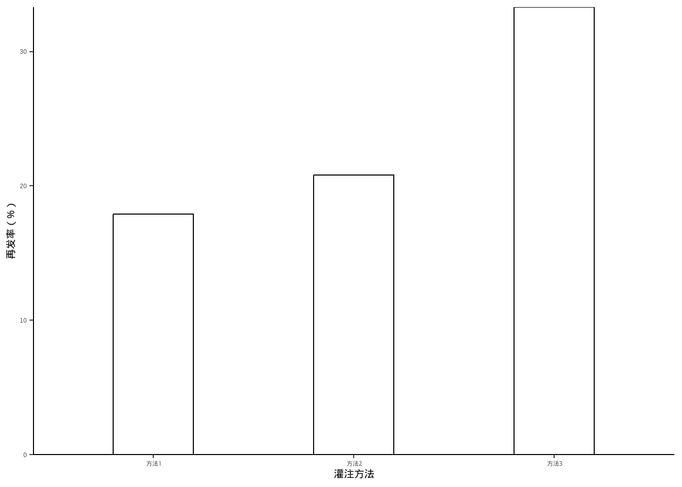
例10-5。分组条形图。
library(haven)
data10_5 <- haven::read_sav("datasets/例10-05.sav")
data10_5 <- as_factor(data10_5)
data10_5
## # A tibble: 4 × 3
##   year  agent  rate
##   <fct> <fct> <dbl>
## 1 2005  男       75
## 2 2005  女       60
## 3 2010  男       56
## 4 2010 女 53library(ggplot2)
ggplot(data10_5, aes(agent,rate))+
geom_bar(stat = "identity",aes(fill=year),position = "dodge")+
labs(x="性别",y="患龋率(%)",fill="年份")+
scale_y_continuous(expand = c(0,0))+
theme_classic()+
theme(axis.title = element_text(color = "black",size = 15))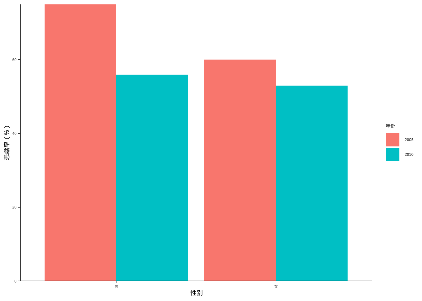
例10-6。饼图。
data10_6 <- data.frame(`失败原因`=c("无菌性松动","感染","假体周围骨折","假体不稳定","其他"),
                       `数量`=c(226,52,22,17,10))

library(dplyr)

data10_6 <- data10_6 %>%
  arrange(desc(`数量`)) %>%
  mutate(`失败原因`=factor(`失败原因`,levels=c("无菌性松动","感染",
                                       "假体周围骨折","假体不稳定","其他"))) %>%
  mutate(prop = round(`数量` / sum(`数量`),2),
         prop = scales::percent(prop))

data10_6
##       失败原因 数量 prop
## 1   无菌性松动  226  69%
## 2         感染   52  16%
## 3 假体周围骨折   22   7%
## 4   假体不稳定   17   5%
## 5 其他 10 3%由于ggplot2的大佬们普遍认为饼图是一种很差劲的图形,所以ggplot2对饼图的支持并不好。
# 默认的大概是这种程度
ggplot(data10_6, aes(x="",y=`数量`,fill=`失败原因`))+
  geom_bar(stat = "identity",width = 1,color="white")+
  geom_text(aes(label = prop),position = position_stack(vjust = 0.5))+
  coord_polar("y", start=0)+
  theme_void()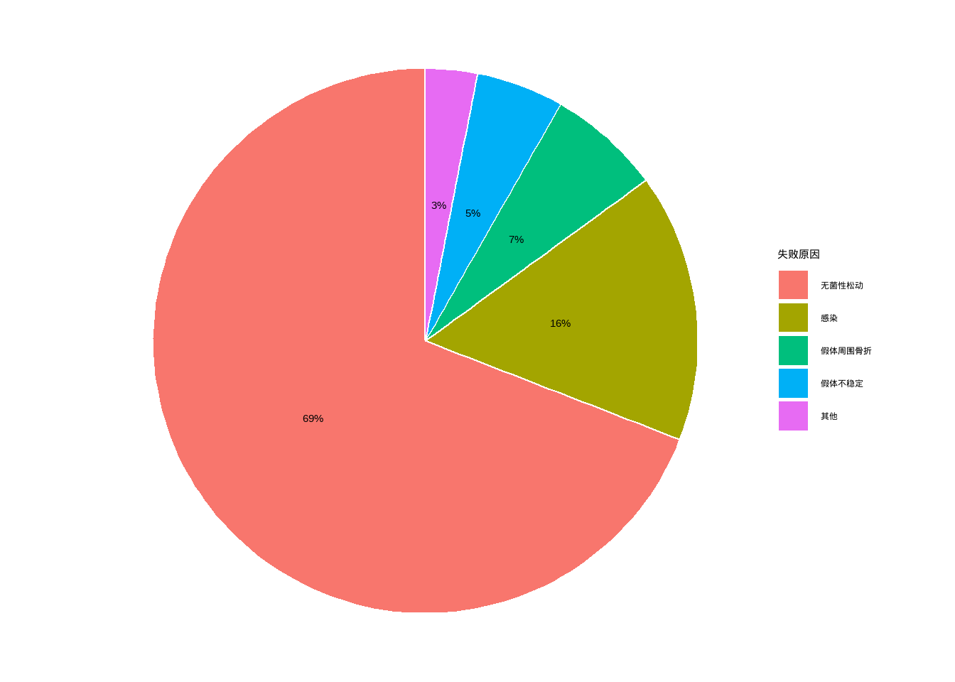
例10-7。百分比条形图。
library(haven)
data10_7 <- haven::read_sav("datasets/例10-07.sav",encoding = "GBK")
data10_7 <- as_factor(data10_7)
data10_7
## # A tibble: 12 × 3
##    year   reason   percent
##    <fct>  <fct>      <dbl>
##  1 1996年 肺炎        23.4
##  2 1996年 早产        14.2
##  3 1996年 出生窒息    14.1
##  4 1996年 腹泻         5.6
##  5 1996年 意外窒息     4.1
##  6 1996年 其它        38.6
##  7 2000年 肺炎        19.5
##  8 2000年 早产        17
##  9 2000年 出生窒息    15.9
## 10 2000年 腹泻         4.9
## 11 2000年 意外窒息     3.7
## 12 2000年 其它 39library(scales)
ggplot(data10_7, aes(year, percent, fill=reason))+
geom_bar(stat = "identity",position = "stack",width = 0.5,color="black")+
labs(fill="",x="",y="")+
scale_y_continuous(labels = percent_format(scale = 1))+
guides(fill=guide_legend(reverse = T))+
theme_bw()+
theme(axis.text = element_text(size = 18, colour = "black"),
legend.text = element_text(size = 18, colour = "black"),
legend.position = "bottom")+
coord_flip()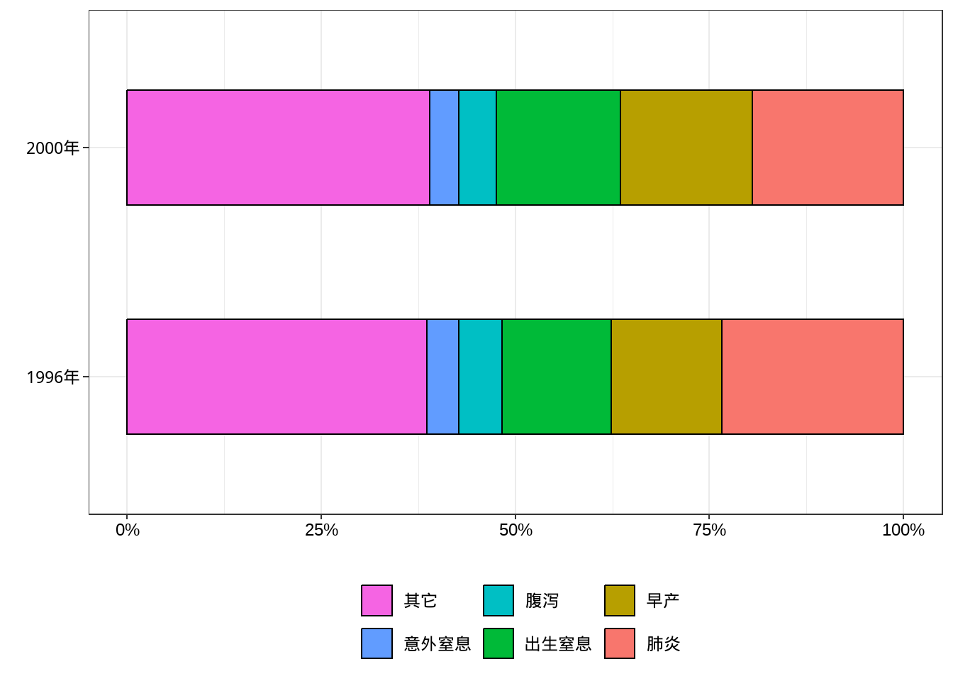
#ggsave("xxxx.png",width=10,height=5,dpi=300)例10-8。折线图。
library(haven)
data10_8 <- haven::read_sav("datasets/例10-08.sav",encoding = "GBK")
data10_8 <- as_factor(data10_8)
data10_8
## # A tibble: 10 × 3
##    year  agent counts
##    <fct> <fct>  <dbl>
##  1 2006  男      5500
##  2 2006  女      2500
##  3 2007  男      6000
##  4 2007  女      3000
##  5 2008  男      9000
##  6 2008  女      3500
##  7 2009  男     11000
##  8 2009  女      5000
##  9 2010  男     11000
## 10 2010 女 5000ggplot(data10_8, aes(year,counts))+
geom_line(aes(group = agent,linetype=agent))+
labs(x="年份",y="布氏菌病发病人数",linetype="性别")+
theme_classic()+
theme(axis.text = element_text(size = 18, colour = "black"),
axis.title = element_text(color = "black",size = 18),
legend.text = element_text(size = 18, colour = "black"),
legend.title = element_text(size = 18, colour = "black"))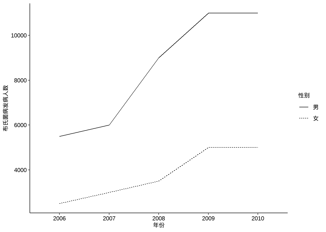
例10-9。点线图。
library(haven)
data10_9 <- haven::read_sav("datasets/例10-09.sav",encoding = "GBK")
data10_9 <- as_factor(data10_9)
data10_9
## # A tibble: 10 × 3
##     year 病型   发病率
##    <dbl> <fct>   <dbl>
##  1  1997 艾滋病 0.0069
##  2  1998 艾滋病 0.0177
##  3  1999 艾滋病 0.0187
##  4  2000 艾滋病 0.0312
##  5  2001 艾滋病 0.0468
##  6  1997 梅毒   3.76
##  7  1998 梅毒   4.58
##  8  1999 梅毒   5.72
##  9  2000 梅毒   6.09
## 10  2001 梅毒   6.27
p1 <- ggplot(data10_9, aes(year,`发病率`))+
geom_line(aes(group = `病型`,linetype=`病型`))+
geom_point(aes(group = `病型`,shape=`病型`),size=4)+
labs(x="年份",y="发病率(1/10万)")+
theme_classic()+
theme(axis.text = element_text(size = 14, colour = "black"),
axis.title = element_text(color = "black",size = 14),
legend.text = element_text(size = 14, colour = "black"),
legend.title = element_text(size = 14, colour = "black"))
p2 <- ggplot(data10_9, aes(year,log10(`发病率`)))+ # 不知道课本取的log几
geom_line(aes(group = `病型`,linetype=`病型`))+
geom_point(aes(group = `病型`,shape=`病型`),size=4)+
labs(x="年份",y="发病率(1/10万)")+
theme_classic()+
theme(axis.text = element_text(size = 14, colour = "black"),
axis.title = element_text(color = "black",size = 14),
legend.text = element_text(size = 14, colour = "black"),
legend.title = element_text(size = 14, colour = "black"))
library(patchwork)
p1+p2+plot_layout(guides = "collect")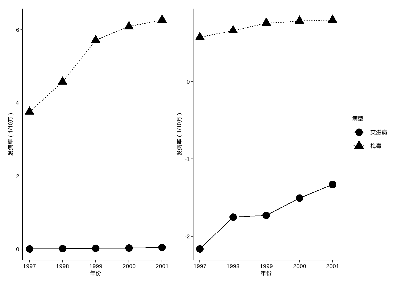
例10-10。直方图。
library(haven)
data10_10 <- haven::read_sav("datasets/例10-10.sav",encoding = "GBK")
data10_10 <- as_factor(data10_10)
data10_10
## # A tibble: 16 × 2
##    age   count
##    <fct> <dbl>
##  1 0-        7
##  2 1-       15
##  3 2-        8
##  4 3-       11
##  5 4-       14
##  6 5-       14
##  7 6-        8
##  8 7-        6
##  9 8-        3
## 10 9-        2
## 11 10-       8
## 12 15-       3
## 13 20-       1
## 14 25-       2
## 15 30-       1
## 16 35-40     1
下面这个其实假的直方图(虽然和课本中的看起来差不多),因为没给原始数据,给的是计数好的数据,所以是用条形图伪装的直方图:
ggplot(data10_10, aes(age,count))+
  geom_bar(stat = "identity",fill="white",color="black",
           width = 1,position = position_dodge(width = 1))+
  labs(x="年龄(岁)",y="每岁病例数")+
  scale_y_continuous(expand = c(0,0))+
  theme_classic()+
  theme(axis.title = element_text(color = "black",size = 15))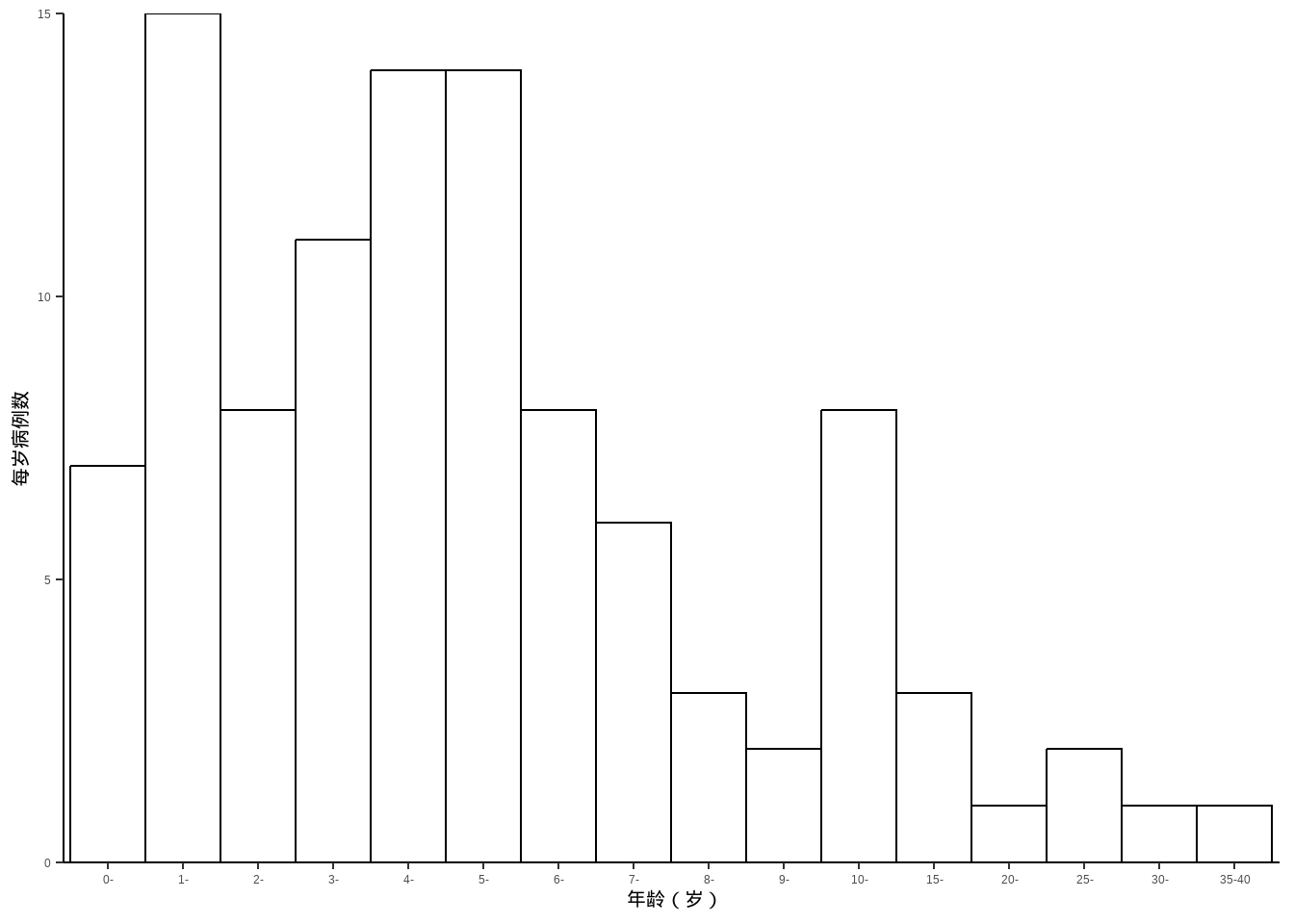
例10-11。地图。没给数据,直接自己编一个。
首先下载中国地图。中国地图下载地址:地图选择器
library(ggplot2)
library(sf)
library(dplyr)

china_map <- st_read("datasets/中华人民共和国.json")
## Reading layer `中华人民共和国' from data source
##   `F:\R_books\medstat_quartobook\datasets\中华人民共和国.json'
##   using driver `GeoJSON'
## Simple feature collection with 35 features and 10 fields
## Geometry type: MULTIPOLYGON
## Dimension:     XY
## Bounding box:  xmin: 73.50235 ymin: 3.397162 xmax: 135.0957 ymax: 53.56327
## Geodetic CRS:  WGS 84
然后给每个省编点数据:
set.seed(123)
china_map <- china_map %>%
  mutate(name_short=substr(name,1,2),
         number = sample(10:100,35,replace=F),
         group = sample(paste0("group",1:5),35,replace=T))

china_map$name_short[c(5,8)] <- c("内蒙古","黑龙江")画图即可,ggplot2画地图非常厉害,下面这个只是非常基础的,可以进行非常多的修改。
ggplot(data = china_map) +
  geom_sf(aes(fill=group)) +
  geom_sf_text(aes(label = name_short),nudge_y = 0,size=2)+
  geom_sf_text(aes(label = number),nudge_y = -1,size=2)+
  theme_minimal()
## Warning in st_point_on_surface.sfc(sf::st_zm(x)): st_point_on_surface may not
## give correct results for longitude/latitude data
## Warning in st_point_on_surface.sfc(sf::st_zm(x)): st_point_on_surface may not
## give correct results for longitude/latitude data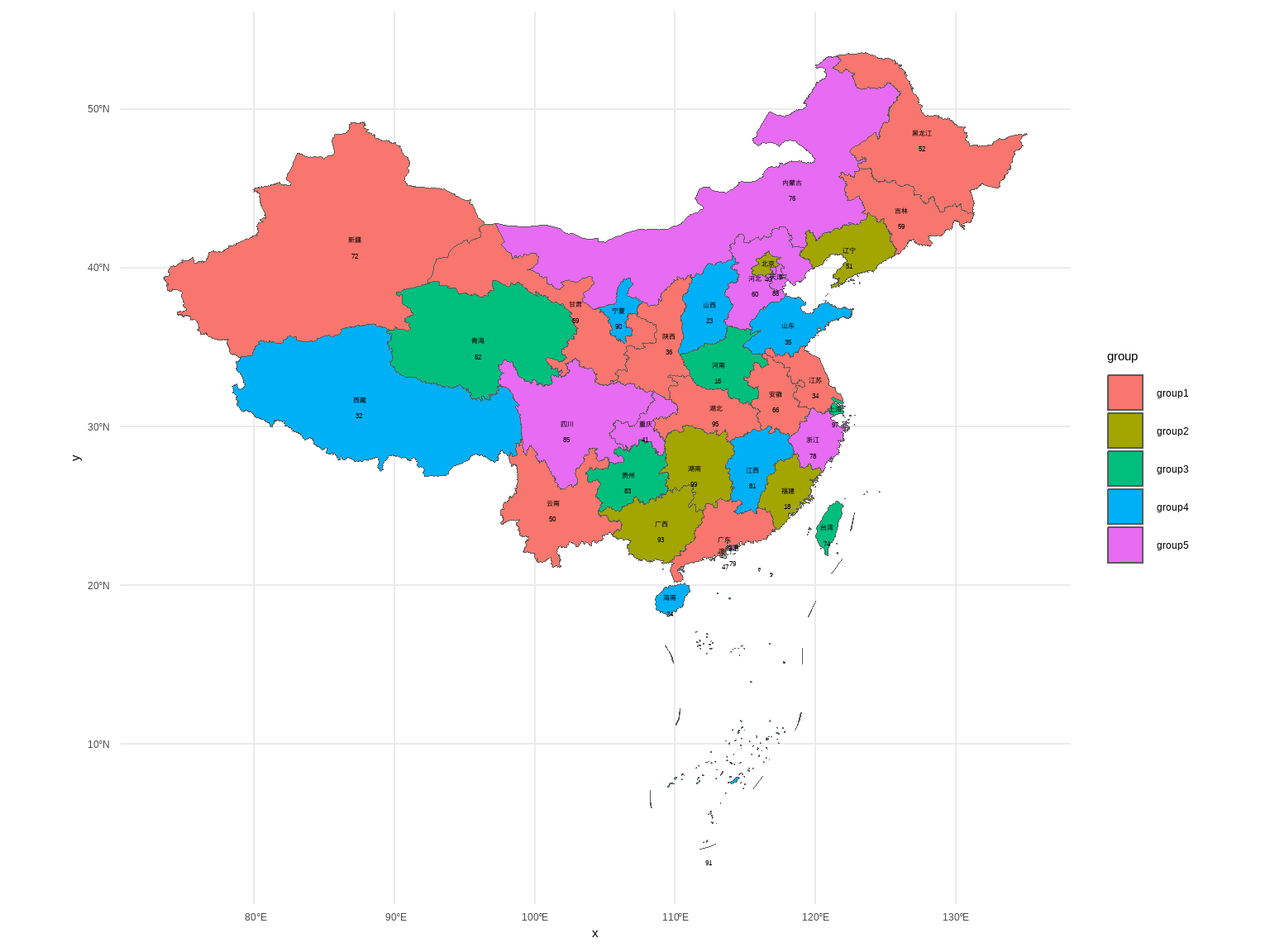
例10-12。箱线图。没给数据,直接用R语言自带的iris数据演示一下。
library(ggplot2)

ggplot(iris, aes(Species,Sepal.Length))+
  stat_boxplot(geom = "errorbar",width = 0.2)+
  geom_boxplot()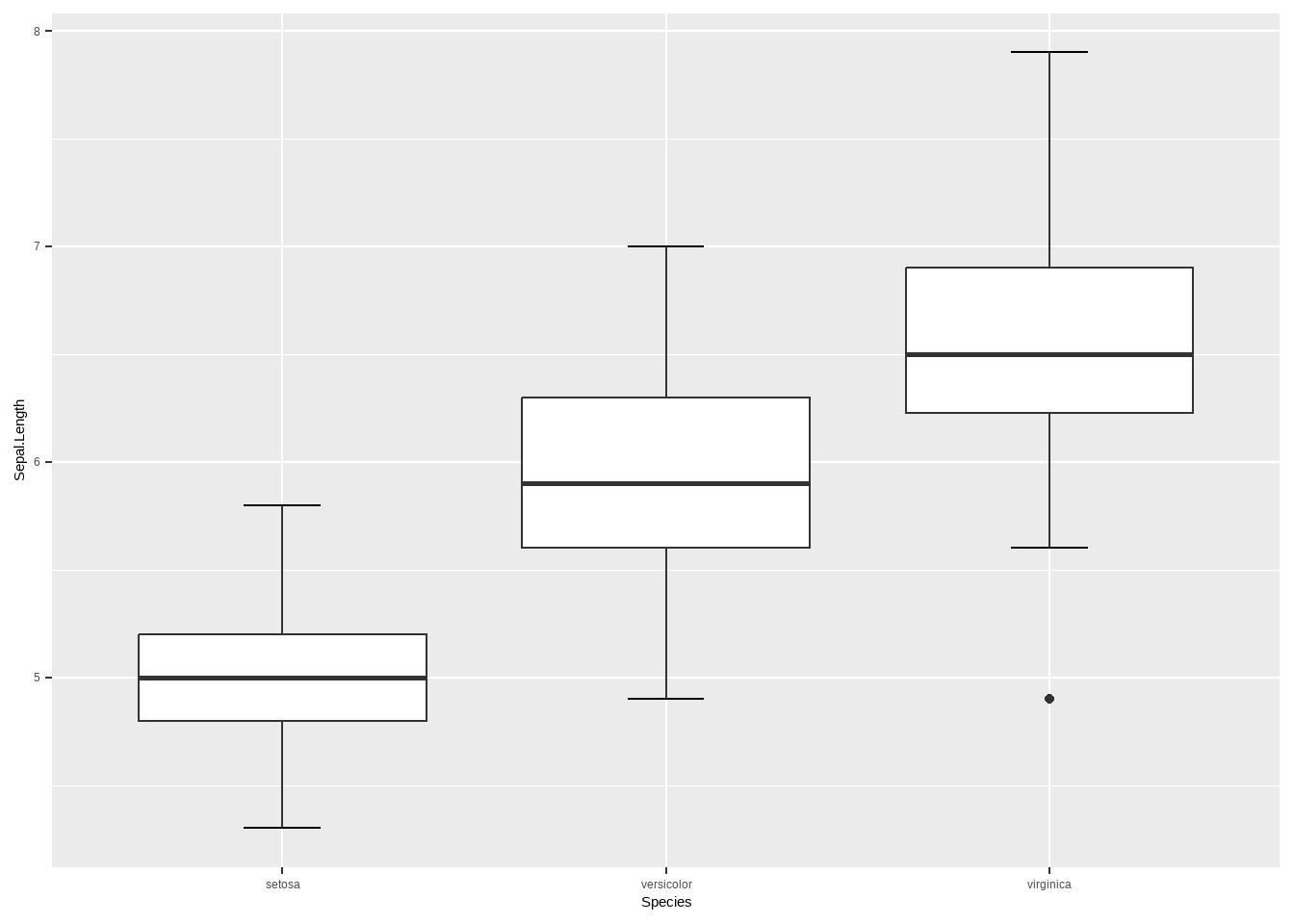
例10-13。茎叶图。
library(haven)
data10_13 <- haven::read_sav("datasets/例10-13.sav",encoding = "GBK")
data10_13 <- as_factor(data10_13)
data10_13
## # A tibble: 138 × 1
##      rbc
##    <dbl>
##  1  3.96
##  2  3.77
##  3  4.63
##  4  4.56
##  5  4.66
##  6  4.61
##  7  4.98
##  8  5.28
##  9  5.11
## 10  4.92
## # ℹ 128 more rows
R自带函数就可以画(但是这个图很少用):
stem(data10_13$rbc,scale = 1)
##
## The decimal point is 1 digit(s) to the left of the |
##
## 30 | 7
## 31 |
## 32 | 17
## 33 | 9
## 34 | 2
## 35 | 299
## 36 | 0124467789
## 37 | 12266679
## 38 | 3399
## 39 | 166667778
## 40 | 11122223344
## 41 | 2234666789
## 42 | 000011133345566666667888999
## 43 | 01223466666
## 44 | 12279
## 45 | 4566677
## 46 | 111366899
## 47 | 15666
## 48 | 139
## 49 | 258
## 50 | 13
## 51 | 12
## 52 | 348
## 53 |
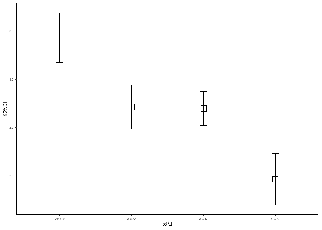
## 54 | 6例10-14。误差条图。
library(haven)
data10_14 <- haven::read_sav("datasets/例10-14.sav",encoding = "GBK")
data10_14 <- as_factor(data10_14)
data10_14
## # A tibble: 120 × 2
##    group     dmdz
##    <fct>    <dbl>
##  1 安慰剂组  3.53
##  2 安慰剂组  4.59
##  3 安慰剂组  4.34
##  4 安慰剂组  2.66
##  5 安慰剂组  3.59
##  6 安慰剂组  3.13
##  7 安慰剂组  2.64
##  8 安慰剂组  2.56
##  9 安慰剂组  3.5
## 10 安慰剂组  3.25
## # ℹ 110 more rows
先计算每个组的均值和可信区间:
95%可信区间的计算:均值±1.96*标准误,见课本第一章第三节:总体均数的估计
library(dplyr)

data10_14_1 <- data10_14 %>%
  group_by(group) %>%
  summarise(mm = mean(dmdz),
            lower = mm - 1.96*(sd(dmdz)/sqrt(30)),
            upper = mm + 1.96*(sd(dmdz)/sqrt(30)))
data10_14_1
## # A tibble: 4 × 4
##   group       mm lower upper
##   <fct>    <dbl> <dbl> <dbl>
## 1 安慰剂组  3.43  3.17  3.69
## 2 新药2.4   2.72  2.49  2.94
## 3 新药4.8   2.70  2.52  2.88
## 4 新药7.2 1.97 1.70 2.23ggplot(data10_14_1)+
geom_point(aes(group,mm),size=4,shape=0)+
geom_errorbar(aes(x=group,ymin=lower,ymax=upper),
width=0.1)+
theme_classic()+
labs(x="分组",y="95%CI")+
theme_classic()+
theme(axis.title = element_text(color = "black",size = 15))