test1<-c(60,142,195,80,242,220,190,25,198,38,236,95)
test2<-c(76,152,243,82,240,220,205,38,243,44,190,100)6 秩转换的非参数检验
6.1 配对样本比较的Wilcoxon符号秩检验
英文名字:wilcoxon signed-rank test,即符号秩检验。
使用课本例8-1的数据,自己手动摘录:
两列数据,和配对t检验的数据结果完全一样。
简单看一下数据情况:
boxplot(test1,test2)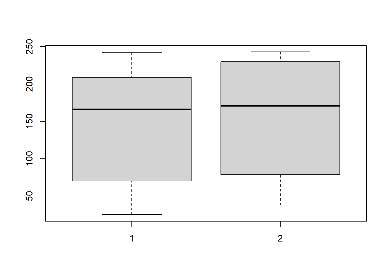
进行秩和检验:
wilcox.test(test1,test2,paired = T,alternative = "two.sided",exact = F)
##
##  Wilcoxon signed rank test with continuity correction
##
## data:  test1 and test2
## V = 11.5, p-value = 0.06175
## alternative hypothesis: true location shift is not equal to 0
结果和课本一致!
注意
wilcox.test在R4.4.0及以后不再支持在公式形式中使用paired参数,所以如果你的R版本在4.4.0及以后的,在公式形式中使用paired参数会得到以下报错:cannot use 'paired' in formula method。逆天更新!!
6.2 两独立样本比较的Wilcoxon秩和检验
英文名字:wilcoxon rank sum test,即秩和检验。
根据课本上的说法,wilcoxon rank sum test 和 mann-whitney U test 并不完全是一个东西。
和两样本t检验的数据格式完全一样!
使用课本例8-3的数据,自己手动摘录。
RD1<-c(2.78,3.23,4.20,4.87,5.12,6.21,7.18,8.05,8.56,9.60)
RD2<-c(3.23,3.50,4.04,4.15,4.28,4.34,4.47,4.64,4.75,4.82,4.95,5.10)
进行两独立样本比较的Wilcoxon秩和检验:
wilcox.test(RD1,RD2,paired = F, correct = F, exact = F)
##
##  Wilcoxon rank sum test
##
## data:  RD1 and RD2
## W = 86.5, p-value = 0.08049
## alternative hypothesis: true location shift is not equal to 0
结果取单侧检验,还是和课本一致!
6.3 完全随机设计多个样本比较的 Kruskal-Wallis H 检验
6.3.1 多样本比较的kruskal-wallis H检验
使用课本例8-5的数据,手动摘录:
rm(list = ls())
death_rate <- c(32.5,35.5,40.5,46,49,16,20.5,22.5,29,36,6.5,
                9.0,12.5,18,24)
drug <- rep(c("Drug_A","drug_B","drug_C"),each=5)
mydata <- data.frame(death_rate,drug)

str(mydata)
## 'data.frame':    15 obs. of  2 variables:
##  $ death_rate: num  32.5 35.5 40.5 46 49 16 20.5 22.5 29 36 ...
##  $ drug      : chr  "Drug_A" "Drug_A" "Drug_A" "Drug_A" ...
数据一共2列,第1列是死亡率,第2列是药物(3种)。
简单看下数据:
boxplot(death_rate ~ drug, data = mydata)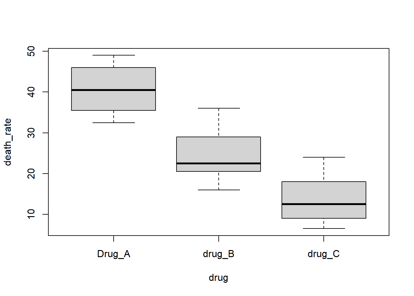
进行 Kruskal-Wallis H 检验:
kruskal.test(death_rate ~ drug, data = mydata)
##
##  Kruskal-Wallis rank sum test
##
## data:  death_rate by drug
## Kruskal-Wallis chi-squared = 9.74, df = 2, p-value = 0.007673
算出来结果和课本一致!
使用课本例8-6的数据,手动摘录:
data8_6 <- data.frame(days=c(2,2,2,3,4,4,4,5,7,7,
                             5,5,6,6,6,7,8,10,12,
                             3,5,6,6,6,7,7,9,10,11,11),
                      type=c(rep("9D",10),rep("11C",9),rep("DSC",11)))
head(data8_6)
##   days type
## 1    2   9D
## 2    2   9D
## 3    2   9D
## 4    3   9D
## 5    4   9D
## 6    4   9D
进行 Kruskal-Wallis H 检验:
kruskal.test(days ~ type, data = data8_6)
##
##  Kruskal-Wallis rank sum test
##
## data:  days by type
## Kruskal-Wallis chi-squared = 9.9405, df = 2, p-value = 0.006941
结果和课本一致(课本中Hc=9.97)。
6.3.2 kruskal-Wallis H检验后的多重比较
例8-8使用的是例8-6的数据。
课本上是使用的 Nemenyi检验,我们使用非参数检验的全能R包:PMCMRplus实现。
library(PMCMRplus)

# 首先要把分类变量因子化
data8_6$type <- factor(data8_6$type)
下面就可以使用 Nemenyi检验了。
# 也可以把kwh检验的结果作为输入
res <- kwAllPairsNemenyiTest(days ~ type, data = data8_6)
## Warning in kwAllPairsNemenyiTest.default(c(2, 2, 2, 3, 4, 4, 4, 5, 7, 7, : Ties
## are present, p-values are not corrected.
summary(res)
##                q value Pr(>|q|)
## 9D - 11C == 0    3.628 0.027794 *
## DSC - 11C == 0   0.177 0.991411
## DSC - 9D == 0    3.998 0.013057 *
得到的数值和课本有差别,但是结论是一样的。
6.4 随记区组设计多个样本比较的Friedman M检验
6.4.1 多个相关样本比较的Friedman M检验
使用课本例8-9的数据:
df <- foreign::read.spss("datasets/例08-09.sav", to.data.frame = T)

str(df)
## 'data.frame':    8 obs. of  4 variables:
##  $ a: num  8.4 11.6 9.4 9.8 8.3 8.6 8.9 7.8
##  $ b: num  9.6 12.7 9.1 8.7 8 9.8 9 8.2
##  $ c: num  9.8 11.8 10.4 9.9 8.6 9.6 10.6 8.5
##  $ d: num  11.7 12 9.8 12 8.6 10.6 11.4 10.8
##  - attr(*, "codepage")= int 65001
数据一共4列,分别是4中不同频率下的反应率。
简单看下数据:
boxplot(df$a,df$b,df$c,df$d)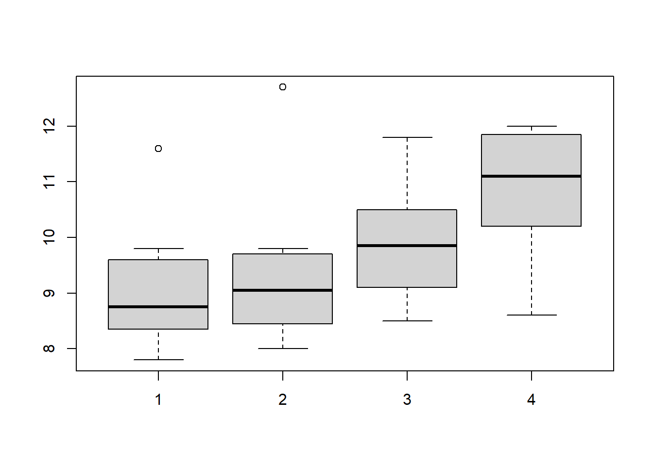
进行 Friedman M 检验前先把数据格式转换一下:
M <- as.matrix(df) # 变成矩阵进行 Friedman M 检验:
friedman.test(M)
##
##  Friedman rank sum test
##
## data:  M
## Friedman chi-squared = 15.152, df = 3, p-value = 0.001691
结果和课本一致!
6.4.2 多个相关样本两两比较的q检验
P126页,多个相关样本两两比较的q检验。课本上说的这个q检验,应该是quade test。
接下来就是使用R语言实现quade-test。但是自带的quade.test()函数不能进行两两比较,还是要借助第三方包。
# 准备数据,也是用的课本例8-9的数据
df <- matrix(
  c(8.4, 11.6, 9.4, 9.8, 8.3, 8.6, 8.9, 7.8,
    9.6, 12.7, 9.1, 8.7, 8, 9.8, 9, 8.2,
    9.8, 11.8, 10.4, 9.9, 8.6, 9.6, 10.6, 8.5,
    11.7, 12, 9.8, 12, 8.6, 10.6, 11.4, 10.8
    ),
  byrow = F, nrow = 8,
  dimnames = list(1:8,LETTERS[1:4])
  )

print(df)
##      A    B    C    D
## 1  8.4  9.6  9.8 11.7
## 2 11.6 12.7 11.8 12.0
## 3  9.4  9.1 10.4  9.8
## 4  9.8  8.7  9.9 12.0
## 5  8.3  8.0  8.6  8.6
## 6  8.6  9.8  9.6 10.6
## 7  8.9  9.0 10.6 11.4
## 8  7.8  8.2  8.5 10.8
先进行 Friedman M检验看看:
friedman.test(df)
##
##  Friedman rank sum test
##
## data:  df
## Friedman chi-squared = 15.152, df = 3, p-value = 0.001691
接下来进行quade检验:
library(PMCMRplus)

quadeAllPairsTest(df, dist = "Normal")
##   A       B       C
## B 0.2200  -       -
## C 0.0017  0.0644  -
## D 1.7e-07 7.7e-05 0.0860
当然也可以有更加详细的结果:
res <- quadeAllPairsTest(df,dist = "Normal")
toTidy(res)
##   group1 group2 statistic      p.value alternative
## 1      B      A  1.226488 2.200150e-01   two.sided
## 2      C      A  3.526154 1.686568e-03   two.sided
## 3      C      B  2.299666 6.440153e-02   two.sided
## 4      D      A  5.549859 1.715396e-07   two.sided
## 5      D      B  4.323371 7.683144e-05   two.sided
## 6      D      C  2.023706 8.600089e-02   two.sided
##                                           method distribution p.adjust.method
## 1 Quade's testwith standard-normal approximation            z            holm
## 2 Quade's testwith standard-normal approximation            z            holm
## 3 Quade's testwith standard-normal approximation            z            holm
## 4 Quade's testwith standard-normal approximation            z            holm
## 5 Quade's testwith standard-normal approximation            z            holm
## 6 Quade's testwith standard-normal approximation            z            holm
这个结果和课本上也不是完全一样,不过不影响结果。还有很多其他的方法可以选择,除了这个quade检验,还可以用Nemenyi等检验方法。