if(!require(devtools)) install.packages("devtools")
devtools::install_github("kassambara/rstatix")

# 或者cran
install.packages("rstatix")13 R语言tidy风格医学统计学
上面的介绍多数是基于R语言自带的函数进行医学统计学分析,下面介绍一个比较现代化、用法也更加简单直接的方法。
提供一个简单直观的管道友好的框架,与整洁的设计理念一致,用于执行基本的统计检验,包括t检验,Wilcoxon检验,方差分析,Kruskal-Wallis和相关性分析。每个分析的输出会自动转换成一个整洁的数据框架,以方便可视化。
附加功能可用于重塑,重新排序,操作和可视化相关矩阵。功能还包括析因实验的分析,包括重复测量设计、析因设计、正交设计等。
可以计算几个效应大小指标,包括方差分析eta平方,t检验的Cohen’s-d和分类变量之间的关联的Cramer’s-v。 该软件包包含用于识别单变量和多变量异常值、评估正态性和方差齐性的辅助函数。
13.1 主要函数
13.1.1 描述性统计
get_summary_stat():计算描述性的统计指标;freq_table(): 分类变量的频率表;get_mode(): 众数;identify_outliers(): 使用boxplot鉴别离群值;mahalanobis_distance(): 计算Mahalanobi距离和离群点;shapiro_test()andmshapiro_test(): 正态性检验.
13.1.2 比较均值
t_test(): 单样本、配对样本、独立样本t检验;wilcox_test(): 单样本、配对样本、独立样本秩和检验;sign_test(): 符号检验;anova_test(): 基于car::Anova()改写,可以做:独立测量、重复测量、混合anova;get_anova_test_table(): 从anova_test()提取结果,可自动执行球形检验.;welch_anova_test(): Welch one-Way ANOVA test. 基于stats::oneway.test()改写;kruskal_test(): kruskal-wallis rank sum test;friedman_test(): Friedman rank sum test;get_comparisons(): 创建需要比较的组;get_pvalue_position: 使用ggplot2添加p值时可自动计算添加坐标
13.1.3 增强R中的ANOVA
factorial_design(): 建立因子化的设计,方便使用car::Anova()进行分析,对于重复测量Anova非常有帮助;anova_summary(): 提取美观的Anova检验的结果,包括从car:Anova()或者stats:aov()中,主要结果包含Anova结果表、一般效应量、和一些假设检验,比如球形检验。
13.1.4 事后检验(post-hoc)
tukey_hsd(): tukey post-hoc tests;dunn_test(): 计算Kruskal-Wallis的成对比较;games_howell_test(): Games-Howell test;emmeans_test(): estimated marginal means
13.1.5 比较比例
prop_test(),pairwise_prop_test()androw_wise_prop_test(). Performs one-sample and two-samples z-test of proportions. Wrappers around the R base function prop.test() but have the advantage of performing pairwise and row-wise z-test of two proportions, the post-hoc tests following a significant chi-square test of homogeneity for 2xc and rx2 contingency tables.fisher_test(),pairwise_fisher_test()androw_wise_fisher_test(): Fisher’s exact test for count data. Wrappers around the R base function fisher.test() but have the advantage of performing pairwise and row-wise fisher tests, the post-hoc tests following a significant chi-square test of homogeneity for 2xc and rx2 contingency tables.chisq_test(),pairwise_chisq_gof_test(),pairwise_chisq_test_against_p(): Performs chi-squared tests, including goodness-of-fit, homogeneity and independence tests.binom_test(),pairwise_binom_test(),pairwise_binom_test_against_p(): Performs exact binomial test and pairwise comparisons following a significant exact multinomial test. Alternative to the chi-square test of goodness-of-fit-test when the sample.multinom_test(): performs an exact multinomial test. Alternative to the chi-square test of goodness-of-fit-test when the sample size is small.mcnemar_test(): performs McNemar chi-squared test to compare paired proportions. Provides pairwise comparisons between multiple groups.cochran_qtest(): extension of the McNemar Chi-squared test for comparing more than two paired proportions.prop_trend_test(): Performs chi-squared test for trend in proportion. This test is also known as Cochran-Armitage trend test
13.1.6 比较方差
levene_test(): Pipe-friendly framework to easily compute Levene’s test for homogeneity of variance across groups.box_m(): Box’s M-test for homogeneity of covariance matrices
13.1.7 计算效应量
cohens_d(): Compute cohen’s d measure of effect size for t-tests.wilcox_effsize(): Compute Wilcoxon effect size (r).eta_squared()andpartial_eta_squared(): Compute effect size for ANOVA.kruskal_effsize(): Compute the effect size for Kruskal-Wallis test as the eta squared based on the H-statistic.friedman_effsize(): Compute the effect size of Friedman test using the Kendall’s W value.cramer_v(): Compute Cramer’s V, which measures the strength of the association between categorical variables
13.1.8 相关性分析
13.1.8.1 计算相关性
cor_test(): correlation test between two or more variables using Pearson, Spearman or Kendall methods.cor_mat(): compute correlation matrix with p-values. Returns a data frame containing the matrix of the correlation coefficients. The output has an attribute named “pvalue”, which contains the matrix of the correlation test p-values.cor_get_pval(): extract a correlation matrix p-values from an object of class cor_mat().cor_pmat(): compute the correlation matrix, but returns only the p-values of the correlation tests.as_cor_mat(): convert a cor_test object into a correlation matrix format.
13.1.8.2 重塑相关矩阵
cor_reorder(): reorder correlation matrix, according to the coefficients, using the hierarchical clustering method.cor_gather(): takes a correlation matrix and collapses (or melt) it into long format data frame (paired list)cor_spread(): spread a long correlation data frame into wide format (correlation matrix).
13.1.8.3 相关矩阵取子集
cor_select(): subset a correlation matrix by selecting variables of interest.pull_triangle(),pull_upper_triangle(),pull_lower_triangle(): pull upper and lower triangular parts of a (correlation) matrix.replace_triangle(),replace_upper_triangle(),replace_lower_triangle(): replace upper and lower triangular parts of a (correlation) matrix.
13.1.8.4 可视化相关矩阵
cor_as_symbols(): replaces the correlation coefficients, in a matrix, by symbols according to the value.cor_plot(): visualize correlation matrix using base plot.cor_mark_significant(): add significance levels to a correlation matrix
13.1.9 添加P值和显著性标记
adjust_pvalue(): add an adjusted p-values column to a data frame containing statistical test p-valuesadd_significance(): add a column containing the p-value significance levelp_round(),p_format(),p_mark_significant(): rounding and formatting p-values
13.1.10 提取统计信息
get_pwc_label(): Extract label from pairwise comparisons.get_test_label(): Extract label from statistical tests.create_test_label(): Create labels from user specified test results
13.1.11 数据处理辅助函数
df_select(),df_arrange(),df_group_by(): wrappers arround dplyr functions for supporting standard and non standard evaluations.df_nest_by(): Nest a tibble data frame using grouping specification. Supports standard and non standard evaluations.df_split_by(): Split a data frame by groups into subsets or data panel. Very similar to the functiondf_nest_by(). The only difference is that, it adds labels to each data subset. Labels are the combination of the grouping variable levels.df_unite(): Unite multiple columns into one.df_unite_factors(): Unite factor columns. First, order factors levels then merge them into one column. The output column is a factor.df_label_both(),df_label_value(): functions to label data frames rows by by one or multiple grouping variables.df_get_var_names(): Returns user specified variable names. Supports standard and non standard evaluation
13.1.12 其他
doo(): alternative to dplyr::do for doing anything. Technically it usesnest()+mutate()+map()to apply arbitrary computation to a grouped data frame.sample_n_by(): sample n rows by group from a tableconvert_as_factor(),set_ref_level(),reorder_levels(): Provides pipe-friendly functions to convert simultaneously multiple variables into a factor variable.make_clean_names(): Pipe-friendly function to make syntactically valid column names (for input data frame) or names (for input vector).counts_to_cases(): converts a contingency table or a data frame of counts into a data frame of individual observations
13.2 安装和加载
加载包:
library(rstatix)
##
## Attaching package: 'rstatix'
## The following object is masked from 'package:stats':
##
##     filter
library(ggpubr)
## Loading required package: ggplot2
13.3 描述性统计
# 指定列
iris %>% get_summary_stats(Sepal.Length, Sepal.Width, type = "full")
## # A tibble: 2 × 13
##   variable        n   min   max median    q1    q3   iqr   mad  mean    sd    se
##   <fct>       <dbl> <dbl> <dbl>  <dbl> <dbl> <dbl> <dbl> <dbl> <dbl> <dbl> <dbl>
## 1 Sepal.Leng…   150   4.3   7.9    5.8   5.1   6.4   1.3 1.04   5.84 0.828 0.068
## 2 Sepal.Width   150   2     4.4    3     2.8   3.3   0.5 0.445  3.06 0.436 0.036
## # ℹ 1 more variable: ci <dbl>
# 所有列
iris %>% get_summary_stats(type = "common")
## # A tibble: 4 × 10
## variable n min max median iqr mean sd se ci
## <fct> <dbl> <dbl> <dbl> <dbl> <dbl> <dbl> <dbl> <dbl> <dbl>
## 1 Sepal.Length 150 4.3 7.9 5.8 1.3 5.84 0.828 0.068 0.134
## 2 Sepal.Width 150 2 4.4 3 0.5 3.06 0.436 0.036 0.07
## 3 Petal.Length 150 1 6.9 4.35 3.5 3.76 1.76 0.144 0.285
## 4 Petal.Width 150 0.1 2.5 1.3 1.5 1.20 0.762 0.062 0.123# 分组展示
iris %>% group_by(Species) %>% get_summary_stats(Sepal.Length, type = "mean_sd")
## # A tibble: 3 × 5
## Species variable n mean sd
## <fct> <fct> <dbl> <dbl> <dbl>
## 1 setosa Sepal.Length 50 5.01 0.352
## 2 versicolor Sepal.Length 50 5.94 0.516
## 3 virginica Sepal.Length 50 6.59 0.636# 众数
get_mode(iris$Sepal.Length)
## [1] 513.4 t检验
以t检验为例。
13.4.1 单样本t检验
还是以之前推文中的例3-5的数据:
df <- foreign::read.spss('datasets/例03-05.sav',to.data.frame = T,
                         reencode = "utf-8")
## re-encoding from utf-8

attributes(df)[4] <- NULL

head(df)
##   no  hb
## 1  1 112
## 2  2 137
## 3  3 129
## 4  4 126
## 5  5  88
## 6  6  90
单样本t检验:
df %>% t_test(hb ~ 1, mu = 140)
## # A tibble: 1 × 7
##   .y.   group1 group2         n statistic    df      p
## * <chr> <chr>  <chr>      <int>     <dbl> <dbl>  <dbl>
## 1 hb 1 null model 36 -2.14 35 0.0397结果和t.test()一样哦!
13.4.2 配对t检验
使用之前推文中的例3-6数据:
library(foreign)
df <- foreign::read.spss('datasets/例03-06.sav',to.data.frame = T,
                         reencode = "utf-8")
## re-encoding from utf-8
attributes(df)[4] <- NULL

head(df)
##   no    x1    x2
## 1  1 0.840 0.580
## 2  2 0.591 0.509
## 3  3 0.674 0.500
## 4  4 0.632 0.316
## 5  5 0.687 0.337
## 6  6 0.978 0.517
进行配对样本t检验:
library(tidyr)
st <- df %>% pivot_longer(cols = 2:3, names_to = "X", values_to = "values") %>%
  t_test(values ~ X, paired = T)

st
## # A tibble: 1 × 8
##   .y.    group1 group2    n1    n2 statistic    df         p
## * <chr>  <chr>  <chr>  <int> <int>     <dbl> <dbl>     <dbl>
## 1 values x1 x2 10 10 7.93 9 0.0000238结果和t.test()也是一样的哦!
可视化也可直接完成!
df %>% pivot_longer(cols = 2:3, names_to = "X", values_to = "values") %>%
  ggpaired(x="X",y="values",color = "X",id="no",line.size = 0.5,line.color = "grey",palette = "lancet")+
  stat_pvalue_manual(st,label = "配对t检验 p = {p}",y.position = 1.3)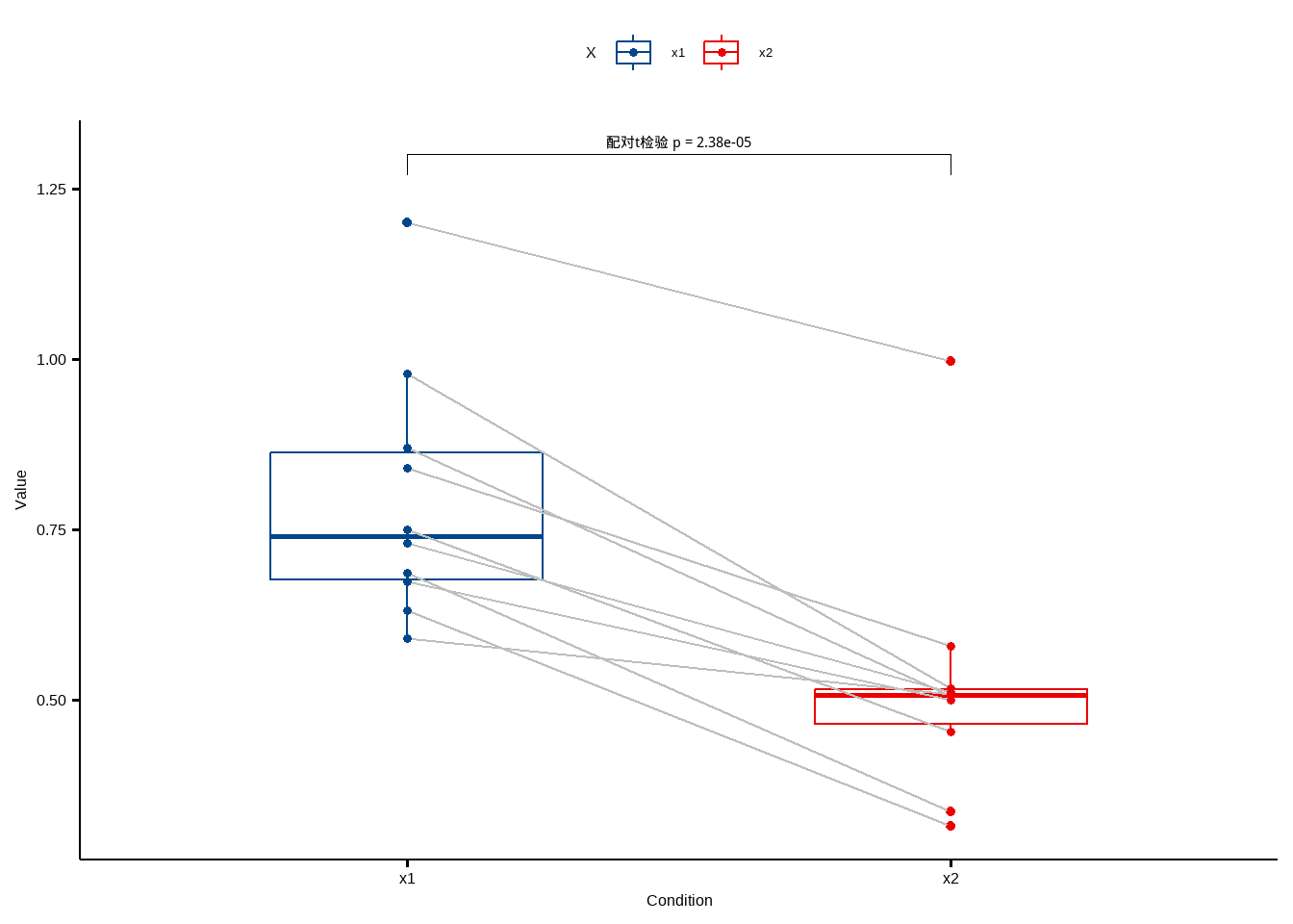
13.4.3 两样本t检验
使用之前推文中的例3-8的数据
df <- foreign::read.spss('datasets/例03-07.sav',to.data.frame = T)
df$group <- c(rep('阿卡波糖',20),rep('拜糖平',20))
attributes(df)[3] <- NULL

head(df)
##   no    x    group
## 1  1 -0.7 阿卡波糖
## 2  2 -5.6 阿卡波糖
## 3  3  2.0 阿卡波糖
## 4  4  2.8 阿卡波糖
## 5  5  0.7 阿卡波糖
## 6  6  3.5 阿卡波糖
进行独立样本t检验:
dt <- df %>% t_test(x ~ group, paired = F)
dt
## # A tibble: 1 × 8
##   .y.   group1   group2    n1    n2 statistic    df     p
## * <chr> <chr>    <chr>  <int> <int>     <dbl> <dbl> <dbl>
## 1 x     阿卡波糖 拜糖平    20    20    -0.642  36.1 0.525
和自带的结果是一样的哦!
顺便可视化一起做了:
ggboxplot(df, x="group", y="x",color = "group", palette = "lancet")+
  stat_pvalue_manual(dt, label = "t-test, p = {p}",y.position = 8)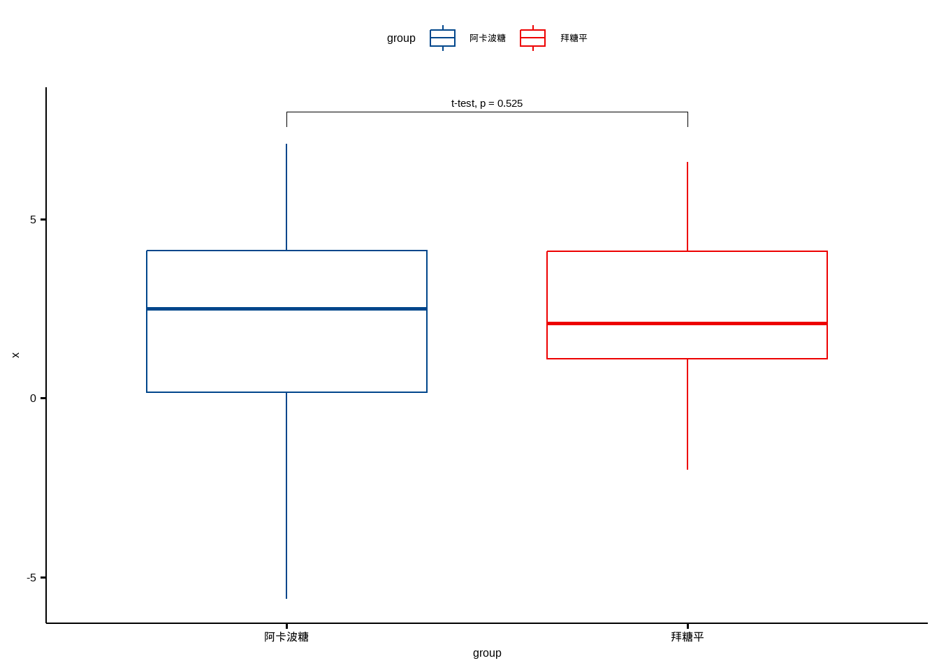
13.4.4 分组后进行比较
df <- ToothGrowth
df$dose <- as.factor(df$dose)
head(df)
##    len supp dose
## 1  4.2   VC  0.5
## 2 11.5   VC  0.5
## 3  7.3   VC  0.5
## 4  5.8   VC  0.5
## 5  6.4   VC  0.5
## 6 10.0   VC  0.5
stat.test <- df %>%
group_by(dose) %>%
t_test(len ~ supp) %>%
adjust_pvalue() %>%
add_significance("p.adj")
stat.test
## # A tibble: 3 × 11
## dose .y. group1 group2 n1 n2 statistic df p p.adj
## <fct> <chr> <chr> <chr> <int> <int> <dbl> <dbl> <dbl> <dbl>
## 1 0.5 len OJ VC 10 10 3.17 15.0 0.00636 0.0127
## 2 1 len OJ VC 10 10 4.03 15.4 0.00104 0.00312
## 3 2 len OJ VC 10 10 -0.0461 14.0 0.964 0.964
## # ℹ 1 more variable: p.adj.signif <chr>ggboxplot(
df, x = "supp", y = "len",
color = "supp", palette = "jco", facet.by = "dose",
ylim = c(0, 40)
) +
stat_pvalue_manual(stat.test, label = "p.adj", y.position = 35)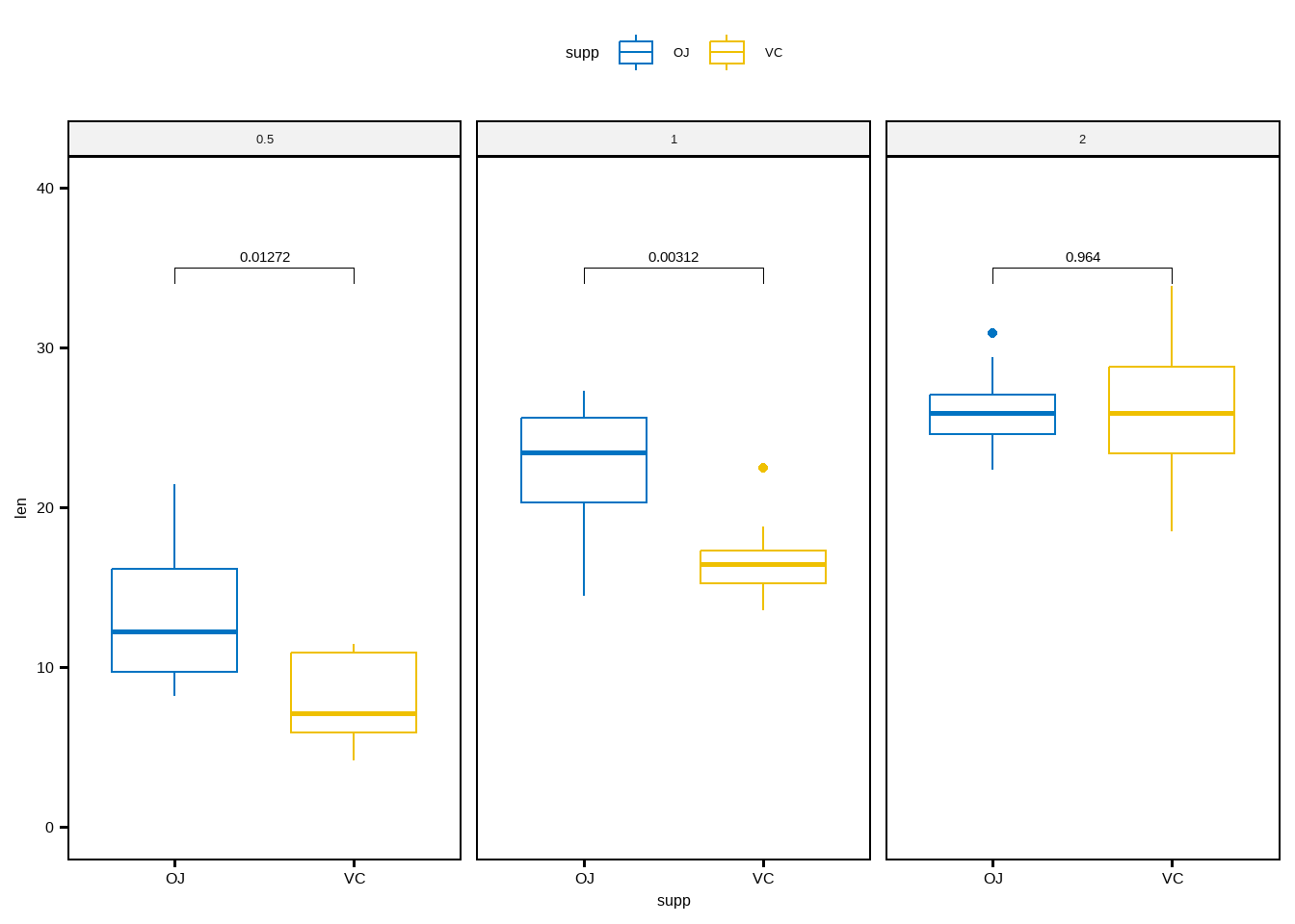
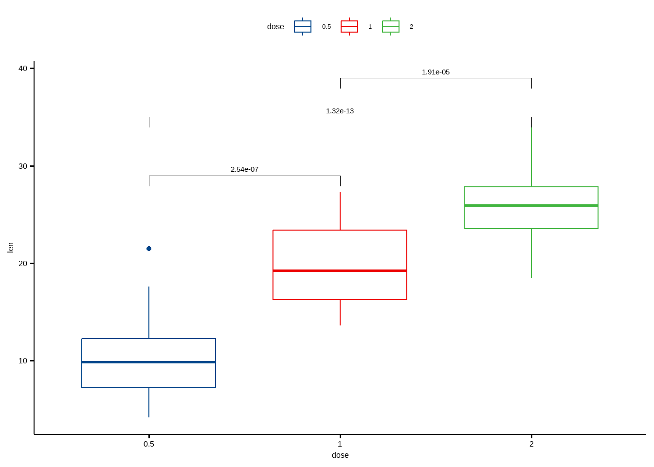
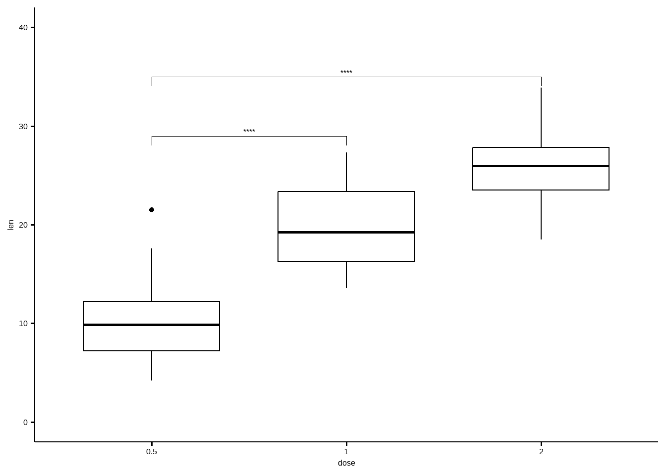
13.4.5 多组间的两两比较
如果有大于2个分组,会自动进行两两比较。
# 两两之间做t检验,自动完成
pairwise.test <- df %>% t_test(len ~ dose)
pairwise.test
## # A tibble: 3 × 10
##   .y.   group1 group2    n1    n2 statistic    df        p    p.adj p.adj.signif
## * <chr> <chr>  <chr>  <int> <int>     <dbl> <dbl>    <dbl>    <dbl> <chr>
## 1 len   0.5    1         20    20     -6.48  38.0 1.27e- 7 2.54e- 7 ****
## 2 len   0.5    2         20    20    -11.8   36.9 4.40e-14 1.32e-13 ****
## 3 len   1      2         20    20     -4.90  37.1 1.91e- 5 1.91e- 5 ****
可视化:
ggboxplot(df, x = "dose", y = "len", color = "dose", palette = "lancet")+
  stat_pvalue_manual(
    pairwise.test, label = "p.adj",
    y.position = c(29, 35, 39)
    )
还可以指定和某一个组进行比较:
# T-test: 都和指定的组进行比较
stat.test <- df %>% t_test(len ~ dose, ref.group = "0.5")
stat.test
## # A tibble: 2 × 10
##   .y.   group1 group2    n1    n2 statistic    df        p    p.adj p.adj.signif
## * <chr> <chr>  <chr>  <int> <int>     <dbl> <dbl>    <dbl>    <dbl> <chr>
## 1 len   0.5    1         20    20     -6.48  38.0 1.27e- 7 1.27e- 7 ****
## 2 len   0.5    2         20    20    -11.8   36.9 4.40e-14 8.80e-14 ****
# Box plot
ggboxplot(df, x = "dose", y = "len", ylim = c(0, 40)) +
stat_pvalue_manual(
stat.test, label = "p.adj.signif",
y.position = c(29, 35)
)
和全部数据进行比较:
stat.test <- df %>% t_test(len ~ dose, ref.group = "all")
stat.test
## # A tibble: 3 × 10
##   .y.   group1 group2    n1    n2 statistic    df         p   p.adj p.adj.signif
## * <chr> <chr>  <chr>  <int> <int>     <dbl> <dbl>     <dbl>   <dbl> <chr>
## 1 len   all    0.5       60    20     5.82   56.4   2.90e-7 8.70e-7 ****
## 2 len   all    1         60    20    -0.660  57.5   5.12e-1 5.12e-1 ns
## 3 len all 2 60 20 -5.61 66.5 4.25e-7 8.70e-7 ****ggboxplot(df, x = "dose", y = "len", fill = "dose",
palette = "lancet", alpha = 0.6) +
stat_pvalue_manual(stat.test, label = "p.adj.signif", y.position = 35) +
geom_hline(yintercept = mean(df$len), linetype = 2)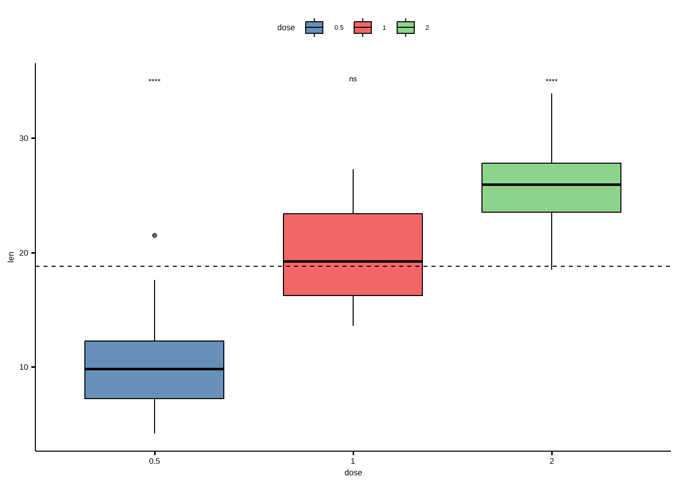
13.5 方差分析
13.5.1 完全随机设计方差分析
使用课本例4-2的数据。
首先是构造数据,本次数据自己从书上摘录。。
trt<-c(rep("group1",30),rep("group2",30),rep("group3",30),rep("group4",30))

weight<-c(3.53,4.59,4.34,2.66,3.59,3.13,3.30,4.04,3.53,3.56,3.85,4.07,1.37,
          3.93,2.33,2.98,4.00,3.55,2.64,2.56,3.50,3.25,2.96,4.30,3.52,3.93,
          4.19,2.96,4.16,2.59,2.42,3.36,4.32,2.34,2.68,2.95,2.36,2.56,2.52,
          2.27,2.98,3.72,2.65,2.22,2.90,1.98,2.63,2.86,2.93,2.17,2.72,1.56,
          3.11,1.81,1.77,2.80,3.57,2.97,4.02,2.31,2.86,2.28,2.39,2.28,2.48,
          2.28,3.48,2.42,2.41,2.66,3.29,2.70,2.66,3.68,2.65,2.66,2.32,2.61,
          3.64,2.58,3.65,3.21,2.23,2.32,2.68,3.04,2.81,3.02,1.97,1.68,0.89,
          1.06,1.08,1.27,1.63,1.89,1.31,2.51,1.88,1.41,3.19,1.92,0.94,2.11,
          2.81,1.98,1.74,2.16,3.37,2.97,1.69,1.19,2.17,2.28,1.72,2.47,1.02,
          2.52,2.10,3.71)

data1<-data.frame(trt,weight)

head(data1)
##      trt weight
## 1 group1   3.53
## 2 group1   4.59
## 3 group1   4.34
## 4 group1   2.66
## 5 group1   3.59
## 6 group1   3.13
进行完全随机设计资料的方差分析:
data1 %>% anova_test(weight ~ trt)
## ANOVA Table (type II tests)
##
##   Effect DFn DFd      F        p p<.05   ges
## 1    trt   3 116 24.884 1.67e-12     * 0.392
13.5.2 随机区组设计资料的方差分析
使用例4-3的数据。
首先是构造数据,本次数据自己从书上摘录。。
weight <- c(0.82,0.65,0.51,0.73,0.54,0.23,0.43,0.34,0.28,0.41,0.21,
            0.31,0.68,0.43,0.24)
block <- c(rep(c("1","2","3","4","5"),each=3))
group <- c(rep(c("A","B","C"),5))

data4_4 <- data.frame(weight,block,group)

head(data4_4)
##   weight block group
## 1   0.82     1     A
## 2   0.65     1     B
## 3   0.51     1     C
## 4   0.73     2     A
## 5   0.54     2     B
## 6   0.23     2     C
数据一共3列,第一列是小白鼠肉瘤重量,第二列是区组因素(5个区组),第三列是分组(一共3组)
进行随机区组设计资料的方差分析:
data4_4 %>% anova_test(weight ~ group + block)
## ANOVA Table (type II tests)
##
##   Effect DFn DFd      F     p p<.05   ges
## 1  group   2   8 11.937 0.004     * 0.749
## 2  block   4   8  5.978 0.016     * 0.749
13.5.3 拉丁方设计方差分析
使用课本例4-5的数据。
首先是构造数据,本次数据自己从书上摘录。。
psize <- c(87,75,81,75,84,66,73,81,87,85,64,79,73,73,74,78,73,77,77,68,
           69,74,76,73,64,64,72,76,70,81,75,77,82,61,82,61)
drug <- c("C","B","E","D","A","F","B","A","D","C","F","E","F","E","B",
          "A","D","C","A","F","C","B","E","D","D","C","F","E","B","A",
          "E","D","A","F","C","B")
col_block <- c(rep(1:6,6))
row_block <- c(rep(1:6,each=6))
mydata <- data.frame(psize,drug,col_block,row_block)
mydata$col_block <- factor(mydata$col_block)
mydata$row_block <- factor(mydata$row_block)
str(mydata)
## 'data.frame':    36 obs. of  4 variables:
##  $ psize    : num  87 75 81 75 84 66 73 81 87 85 ...
##  $ drug     : chr  "C" "B" "E" "D" ...
##  $ col_block: Factor w/ 6 levels "1","2","3","4",..: 1 2 3 4 5 6 1 2 3 4 ...
##  $ row_block: Factor w/ 6 levels "1","2","3","4",..: 1 1 1 1 1 1 2 2 2 2 ...
数据一共4列,第一列是皮肤疱疹大小,第二列是不同药物(处理因素,共5种),第三列是列区组因素,第四列是行区组因素。
进行拉丁方设计的方差分析:
mydata %>% anova_test(psize ~ drug + col_block + row_block)
## ANOVA Table (type II tests)
##
##      Effect DFn DFd     F     p p<.05   ges
## 1      drug   5  20 3.906 0.012     * 0.494
## 2 col_block   5  20 0.500 0.772       0.111
## 3 row_block   5  20 1.466 0.245       0.268
13.5.4 两阶段交叉设计资料方差分析
使用课本例4-6的数据。
首先是构造数据,本次数据自己从书上摘录。。
contain <- c(760,770,860,855,568,602,780,800,960,958,940,952,635,650,440,450,
             528,530,800,803)
phase <- rep(c("phase_1","phase_2"),10)
type <- c("A","B","B","A","A","B","A","B","B","A","B","A","A","B","B","A",
          "A","B","B","A")
testid <- rep(1:10,each=2)
mydata <- data.frame(testid,phase,type,contain)

str(mydata)
## 'data.frame':    20 obs. of  4 variables:
##  $ testid : int  1 1 2 2 3 3 4 4 5 5 ...
##  $ phase  : chr  "phase_1" "phase_2" "phase_1" "phase_2" ...
##  $ type   : chr  "A" "B" "B" "A" ...
##  $ contain: num  760 770 860 855 568 602 780 800 960 958 ...

mydata$testid <- factor(mydata$testid)
数据一共4列,第一列是受试者id,第二列是不同阶段,第三列是测定方法,第四列是测量值。
进行两阶段交叉设计资料方差分析:
mydata %>% anova_test(contain ~ phase + type + testid)
## ANOVA Table (type II tests)
##
##   Effect DFn DFd        F        p p<.05   ges
## 1  phase   1   8    9.925 1.40e-02     * 0.554
## 2   type   1   8    4.019 8.00e-02       0.334
## 3 testid   9   8 1240.195 1.32e-11     * 0.999
结果和课本一致!
13.5.5 析因设计资料的方差分析
使用课本例11-1的数据,自己手动摘录:
df11_1 <- data.frame(
  x1 = rep(c("外膜缝合","束膜缝合"), each = 10),
  x2 = rep(c("缝合1个月","缝合2个月"), each = 5),
  y = c(10,10,40,50,10,30,30,70,60,30,10,20,30,50,30,50,50,70,60,30)
)

str(df11_1)
## 'data.frame':    20 obs. of  3 variables:
##  $ x1: chr  "外膜缝合" "外膜缝合" "外膜缝合" "外膜缝合" ...
##  $ x2: chr  "缝合1个月" "缝合1个月" "缝合1个月" "缝合1个月" ...
##  $ y : num  10 10 40 50 10 30 30 70 60 30 ...
数据一共3列,第1列是缝合方法,第2列是时间,第3列是轴突通过率。
进行析因设计资料的方差分析:
df11_1 %>% anova_test(y ~ x1 * x2)
## ANOVA Table (type II tests)
##
##   Effect DFn DFd     F     p p<.05   ges
## 1     x1   1  16 0.600 0.450       0.036
## 2     x2   1  16 8.067 0.012     * 0.335
## 3  x1:x2   1  16 0.067 0.800       0.004
13.5.6 正交设计资料的方差分析
使用课本例11-4的数据
df11_4 <- data.frame(
  a = rep(c("5度","25度"),each = 4),
  b = rep(c(0.5, 5.0), each = 2),
  c = c(10, 30),
  d = c(6.0, 8.0,8.0,6.0,8.0,6.0,6.0,8.0),
  x = c(86,95,91,94,91,96,83,88)
)

df11_4$a <- factor(df11_4$a)
df11_4$b <- factor(df11_4$b)
df11_4$c <- factor(df11_4$c)
df11_4$d <- factor(df11_4$d)

str(df11_4)
## 'data.frame':    8 obs. of  5 variables:
##  $ a: Factor w/ 2 levels "25度","5度": 2 2 2 2 1 1 1 1
##  $ b: Factor w/ 2 levels "0.5","5": 1 1 2 2 1 1 2 2
##  $ c: Factor w/ 2 levels "10","30": 1 2 1 2 1 2 1 2
##  $ d: Factor w/ 2 levels "6","8": 1 2 2 1 2 1 1 2
##  $ x: num  86 95 91 94 91 96 83 88
进行正交设计资料的方差分析:
df11_4 %>% anova_test(x ~ a + b + c + d + a * b)
## ANOVA Table (type II tests)
##
##   Effect DFn DFd    F     p p<.05   ges
## 1      a   1   2  3.2 0.216       0.615
## 2      b   1   2  7.2 0.115       0.783
## 3      c   1   2 24.2 0.039     * 0.924
## 4      d   1   2  1.8 0.312       0.474
## 5    a:b   1   2 20.0 0.047     * 0.909
13.5.7 重复测量数据两因素两水平的方差分析
使用课本例12-1的数据,直接读取:
df12_1 <- foreign::read.spss("datasets/12-1.sav", to.data.frame = T)
## re-encoding from CP936

str(df12_1)
## 'data.frame':    20 obs. of  5 variables:
##  $ n    : num  1 2 3 4 5 6 7 8 9 10 ...
##  $ x1   : num  130 124 136 128 122 118 116 138 126 124 ...
##  $ x2   : num  114 110 126 116 102 100 98 122 108 106 ...
##  $ group: Factor w/ 2 levels "处理组","对照组": 1 1 1 1 1 1 1 1 1 1 ...
##  $ d    : num  16 14 10 12 20 18 18 16 18 18 ...
##  - attr(*, "variable.labels")= Named chr [1:5] "编号" "治疗前血压" "治疗后血压" "组别" ...
##   ..- attr(*, "names")= chr [1:5] "n" "x1" "x2" "group" ...
##  - attr(*, "codepage")= int 936
数据一共5列(第5列是自己算出来的,其实原始数据只有4列),第1 列是编号,第2列是治疗前血压,第3例是治疗后血压,第4列是分组,第5列是血压前后差值。
进行重复测量数据两因素两水平的方差分析前,先把数据转换一下格式:
suppressMessages(library(tidyverse))
df12_11 <-
  df12_1[,1:4] %>%
  pivot_longer(cols = 2:3,names_to = "time",values_to = "hp") %>%
  mutate_if(is.character, as.factor)

df12_11$n <- factor(df12_11$n)

str(df12_11)
## tibble [40 × 4] (S3: tbl_df/tbl/data.frame)
##  $ n    : Factor w/ 20 levels "1","2","3","4",..: 1 1 2 2 3 3 4 4 5 5 ...
##  $ group: Factor w/ 2 levels "处理组","对照组": 1 1 1 1 1 1 1 1 1 1 ...
##  $ time : Factor w/ 2 levels "x1","x2": 1 2 1 2 1 2 1 2 1 2 ...
##  $ hp   : num [1:40] 130 114 124 110 136 126 128 116 122 102 ...
进行重复测量数据两因素两水平的方差分析:
hp是因变量,time是测量时间(治疗前和治疗后各测量一次),group是分组因素(两种治疗方法),n是受试者编号
df12_11 %>% anova_test(hp ~ time * group + Error(n/time))
## ANOVA Table (type II tests)
##
##       Effect DFn DFd      F        p p<.05   ges
## 1      group   1  18  1.574 2.26e-01       0.071
## 2       time   1  18 55.008 7.08e-07     * 0.278
## 3 group:time   1  18 18.771 4.01e-04     * 0.116
这个结果也是和课本一样的,只不过没有显示组内误差的情况!
13.5.8 重复测量数据两因素多水平的分析
使用课本例12-3的数据,直接读取:
df12_3 <- foreign::read.spss("datasets/例12-03.sav",to.data.frame = T)

str(df12_3)
## 'data.frame':    15 obs. of  7 variables:
##  $ No   : num  1 2 3 4 5 6 7 8 9 10 ...
##  $ group: Factor w/ 3 levels "A","B","C": 1 1 1 1 1 2 2 2 2 2 ...
##  $ t0   : num  120 118 119 121 127 121 122 128 117 118 ...
##  $ t1   : num  108 109 112 112 121 120 121 129 115 114 ...
##  $ t2   : num  112 115 119 119 127 118 119 126 111 116 ...
##  $ t3   : num  120 126 124 126 133 131 129 135 123 123 ...
##  $ t4   : num  117 123 118 120 126 137 133 142 131 133 ...
##  - attr(*, "variable.labels")= Named chr [1:7] "\xd0\xf2\xba\xc5" "\xd7\xe9\xb1\xf0" "" "" ...
##   ..- attr(*, "names")= chr [1:7] "No" "group" "t0" "t1" ...
数据一共7列,第1列是患者编号,第2列是诱导方法(3种),第3-7列是5个时间点的血压。
首先转换数据格式:
library(tidyverse)

df12_31 <- df12_3 %>%
  pivot_longer(cols = 3:7, names_to = "times", values_to = "hp")

df12_31$No <- factor(df12_31$No)
df12_31$times <- factor(df12_31$times)

str(df12_31)
## tibble [75 × 4] (S3: tbl_df/tbl/data.frame)
##  $ No   : Factor w/ 15 levels "1","2","3","4",..: 1 1 1 1 1 2 2 2 2 2 ...
##  $ group: Factor w/ 3 levels "A","B","C": 1 1 1 1 1 1 1 1 1 1 ...
##  $ times: Factor w/ 5 levels "t0","t1","t2",..: 1 2 3 4 5 1 2 3 4 5 ...
##  $ hp   : num [1:75] 120 108 112 120 117 118 109 115 126 123 ...
进行重复测量两因素多水平的方差分析:
df12_31 %>% anova_test(hp ~ times * group + Error(No/(times)))
## ANOVA Table (type II tests)
##
## $ANOVA
##        Effect DFn DFd       F        p p<.05   ges
## 1       group   2  12   5.783 1.70e-02     * 0.430
## 2       times   4  48 106.558 3.02e-23     * 0.659
## 3 group:times   8  48  19.101 1.62e-12     * 0.409
##
## $`Mauchly's Test for Sphericity`
##        Effect     W     p p<.05
## 1       times 0.293 0.178
## 2 group:times 0.293 0.178
##
## $`Sphericity Corrections`
##        Effect   GGe      DF[GG]    p[GG] p[GG]<.05   HFe      DF[HF]    p[HF]
## 1       times 0.679 2.71, 32.58 1.87e-16         * 0.896 3.59, 43.03 4.65e-21
## 2 group:times 0.679 5.43, 32.58 4.26e-09         * 0.896 7.17, 43.03 2.04e-11
##   p[HF]<.05
## 1         *
## 2         *
这个结果也是和课本一样的,而且直接给出了球形检验的结果!非常方便。
13.6 相关分析
以R语言自带的mtcars数据集为例。
mydata <- mtcars %>%
  select(mpg, disp, hp, drat, wt, qsec)

head(mydata)
##                    mpg disp  hp drat    wt  qsec
## Mazda RX4         21.0  160 110 3.90 2.620 16.46
## Mazda RX4 Wag     21.0  160 110 3.90 2.875 17.02
## Datsun 710        22.8  108  93 3.85 2.320 18.61
## Hornet 4 Drive    21.4  258 110 3.08 3.215 19.44
## Hornet Sportabout 18.7  360 175 3.15 3.440 17.02
## Valiant           18.1  225 105 2.76 3.460 20.22
13.6.1 两个变量
mydata %>% cor_test(wt, mpg, method = "pearson")
## # A tibble: 1 × 8
##   var1  var2    cor statistic        p conf.low conf.high method
##   <chr> <chr> <dbl>     <dbl>    <dbl>    <dbl>     <dbl> <chr>
## 1 wt    mpg   -0.87     -9.56 1.29e-10   -0.934    -0.744 Pearson
13.6.2 一个变量和其他所有变量
mydata %>% cor_test(mpg, method = "pearson")
## # A tibble: 5 × 8
##   var1  var2    cor statistic        p conf.low conf.high method
##   <chr> <chr> <dbl>     <dbl>    <dbl>    <dbl>     <dbl> <chr>
## 1 mpg   disp  -0.85     -8.75 9.38e-10  -0.923     -0.708 Pearson
## 2 mpg   hp    -0.78     -6.74 1.79e- 7  -0.885     -0.586 Pearson
## 3 mpg   drat   0.68      5.10 1.78e- 5   0.436      0.832 Pearson
## 4 mpg   wt    -0.87     -9.56 1.29e-10  -0.934     -0.744 Pearson
## 5 mpg   qsec   0.42      2.53 1.71e- 2   0.0820     0.670 Pearson
13.6.3 所有变量间两两相关性
mydata %>% cor_test(method = "pearson")
## # A tibble: 36 × 8
##    var1  var2    cor statistic        p conf.low conf.high method
##    <chr> <chr> <dbl>     <dbl>    <dbl>    <dbl>     <dbl> <chr>
##  1 mpg   mpg    1       Inf    0          1          1     Pearson
##  2 mpg   disp  -0.85     -8.75 9.38e-10  -0.923     -0.708 Pearson
##  3 mpg   hp    -0.78     -6.74 1.79e- 7  -0.885     -0.586 Pearson
##  4 mpg   drat   0.68      5.10 1.78e- 5   0.436      0.832 Pearson
##  5 mpg   wt    -0.87     -9.56 1.29e-10  -0.934     -0.744 Pearson
##  6 mpg   qsec   0.42      2.53 1.71e- 2   0.0820     0.670 Pearson
##  7 disp  mpg   -0.85     -8.75 9.38e-10  -0.923     -0.708 Pearson
##  8 disp  disp   1       Inf    0          1          1     Pearson
##  9 disp  hp     0.79      7.08 7.14e- 8   0.611      0.893 Pearson
## 10 disp  drat  -0.71     -5.53 5.28e- 6  -0.849     -0.481 Pearson
## # ℹ 26 more rows
可以看到所有的输出都是整洁格式的,而且都给出了详细的统计值。
13.6.4 相关矩阵
当然也提供了相关矩阵的方法。
cor.mat <- mydata %>% cor_mat()

cor.mat
## # A tibble: 6 × 7
##   rowname   mpg  disp    hp   drat    wt   qsec
## * <chr>   <dbl> <dbl> <dbl>  <dbl> <dbl>  <dbl>
## 1 mpg      1    -0.85 -0.78  0.68  -0.87  0.42
## 2 disp    -0.85  1     0.79 -0.71   0.89 -0.43
## 3 hp      -0.78  0.79  1    -0.45   0.66 -0.71
## 4 drat     0.68 -0.71 -0.45  1     -0.71  0.091
## 5 wt      -0.87  0.89  0.66 -0.71   1    -0.17
## 6 qsec     0.42 -0.43 -0.71  0.091 -0.17  1
展示P值矩阵:
cor.mat %>% cor_get_pval()
## # A tibble: 6 × 7
##   rowname      mpg     disp           hp       drat        wt       qsec
##   <chr>      <dbl>    <dbl>        <dbl>      <dbl>     <dbl>      <dbl>
## 1 mpg     0        9.38e-10 0.000000179  0.0000178  1.29e- 10 0.0171
## 2 disp    9.38e-10 0        0.0000000714 0.00000528 1.22e- 11 0.0131
## 3 hp      1.79e- 7 7.14e- 8 0            0.00999    4.15e-  5 0.00000577
## 4 drat    1.78e- 5 5.28e- 6 0.00999      0          4.78e-  6 0.62
## 5 wt      1.29e-10 1.22e-11 0.0000415    0.00000478 2.27e-236 0.339
## 6 qsec    1.71e- 2 1.31e- 2 0.00000577   0.62       3.39e-  1 0
使用*代替p值:
cor.mat %>% cor_as_symbols() %>% pull_lower_triangle()
##   rowname mpg disp hp drat wt qsec
## 1     mpg
## 2    disp   *
## 3      hp   *    *
## 4    drat   +    +  .
## 5      wt   *    *  +    +
## 6    qsec   .    .  +
星号和相关性一起显示:
cor.mat %>% cor_mark_significant()
##   rowname       mpg      disp        hp      drat    wt qsec
## 1     mpg
## 2    disp -0.85****
## 3      hp -0.78****  0.79****
## 4    drat  0.68**** -0.71****   -0.45**
## 5      wt -0.87****  0.89****  0.66**** -0.71****
## 6    qsec     0.42*    -0.43* -0.71****     0.091 -0.17
简单的可视化:
cor.mat %>% cor_reorder() %>% cor_plot()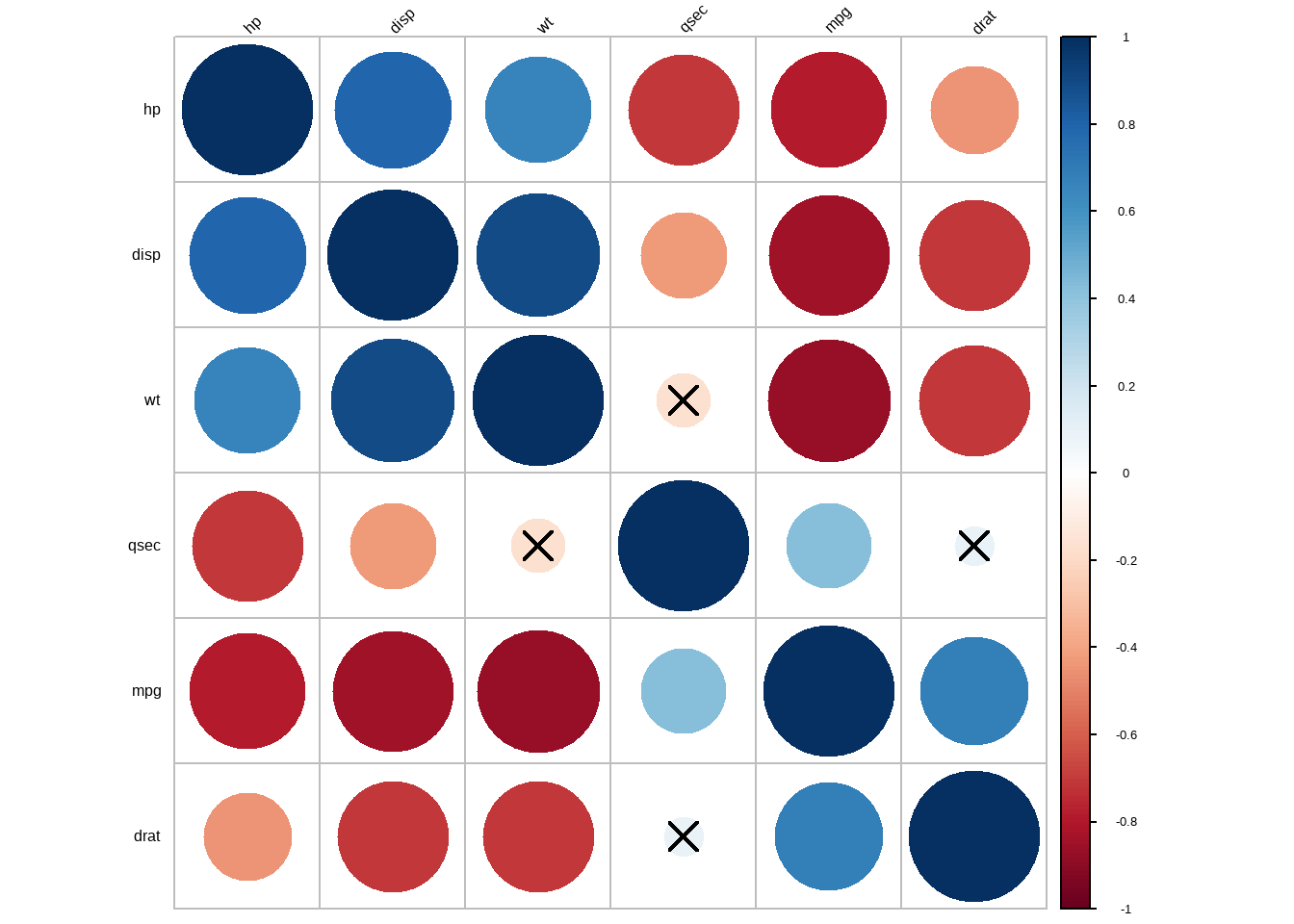
这个图明显是使用corrplot包画出来的,可以直接使用此包画出更好看的图,我的公众号中已有专门介绍corrplot包的推文!
13.7 秩和检验
协方差分析、裂区设计、嵌套设计、都支持!语法完全一样。结果也一样。
13.7.1 配对样本比较的Wilcoxon符号秩检验
课本例8-1的数据
test1<-c(60,142,195,80,242,220,190,25,198,38,236,95)
test2<-c(76,152,243,82,240,220,205,38,243,44,190,100)

df <- data.frame(y=c(test1,test2),group=factor(rep(c(1,2),each=12)))
str(df)
## 'data.frame':    24 obs. of  2 variables:
##  $ y    : num  60 142 195 80 242 220 190 25 198 38 ...
## $ group: Factor w/ 2 levels "1","2": 1 1 1 1 1 1 1 1 1 1 ...没有correct选项
df %>% wilcox_test(y ~ group,paired = T,exact = F)
## # A tibble: 1 × 7
##   .y.   group1 group2    n1    n2 statistic      p
## * <chr> <chr>  <chr>  <int> <int>     <dbl>  <dbl>
## 1 y 1 2 12 12 11.5 0.0618wilcox.test(y ~ group, data = df,paired=T,exact=F,correct=F)
##
## Wilcoxon signed rank test
##
## data: y by group
## V = 11.5, p-value = 0.05581
## alternative hypothesis: true location shift is not equal to 013.7.2 两独立样本比较的Wilcoxon符号秩检验
RD1<-c(2.78,3.23,4.20,4.87,5.12,6.21,7.18,8.05,8.56,9.60)
RD2<-c(3.23,3.50,4.04,4.15,4.28,4.34,4.47,4.64,4.75,4.82,4.95,5.10)

df <- data.frame(y=c(RD1,RD2),group=factor(c(rep(1,10),rep(2,12))))
str(df)
## 'data.frame':    22 obs. of  2 variables:
##  $ y    : num  2.78 3.23 4.2 4.87 5.12 6.21 7.18 8.05 8.56 9.6 ...
## $ group: Factor w/ 2 levels "1","2": 1 1 1 1 1 1 1 1 1 1 ...wilcox.test(RD1,RD2,paired = F, correct = F)
## Warning in wilcox.test.default(RD1, RD2, paired = F, correct = F): cannot
## compute exact p-value with ties
##
## Wilcoxon rank sum test
##
## data: RD1 and RD2
## W = 86.5, p-value = 0.08049
## alternative hypothesis: true location shift is not equal to 0df %>% wilcox_test(y~group)
## # A tibble: 1 × 7
## .y. group1 group2 n1 n2 statistic p
## * <chr> <chr> <chr> <int> <int> <dbl> <dbl>
## 1 y 1 2 10 12 86.5 0.086413.7.3 完全随机设计多个样本比较的 Kruskal-Wallis H 检验
rm(list = ls())
death_rate <- c(32.5,35.5,40.5,46,49,16,20.5,22.5,29,36,6.5,
                9.0,12.5,18,24)
drug <- rep(c("Drug_A","drug_B","drug_C"),each=5)
mydata <- data.frame(death_rate,drug)

str(mydata)
## 'data.frame':    15 obs. of  2 variables:
##  $ death_rate: num  32.5 35.5 40.5 46 49 16 20.5 22.5 29 36 ...
## $ drug : chr "Drug_A" "Drug_A" "Drug_A" "Drug_A" ...kruskal.test(death_rate ~ drug, data = mydata)
##
## Kruskal-Wallis rank sum test
##
## data: death_rate by drug
## Kruskal-Wallis chi-squared = 9.74, df = 2, p-value = 0.007673mydata %>% kruskal_test(death_rate ~ drug)
## # A tibble: 1 × 6
## .y. n statistic df p method
## * <chr> <int> <dbl> <int> <dbl> <chr>
## 1 death_rate 15 9.74 2 0.00767 Kruskal-Wallis13.7.4 随记区组设计多个样本比较的 Friedman M 检验
13.8 卡方检验
13.8.1 四格表资料的卡方检验
ID<-seq(1,200)
treat<-c(rep("treated",104),rep("placebo",96))
treat<- factor(treat)
impro<-c(rep("marked",99),rep("none",5),rep("marked",75),rep("none",21))
impro<-as.factor(impro)
data1<-data.frame(ID,treat,impro)

str(data1)
## 'data.frame':    200 obs. of  3 variables:
##  $ ID   : int  1 2 3 4 5 6 7 8 9 10 ...
##  $ treat: Factor w/ 2 levels "placebo","treated": 2 2 2 2 2 2 2 2 2 2 ...
## $ impro: Factor w/ 2 levels "marked","none": 1 1 1 1 1 1 1 1 1 1 ...library(gmodels)
CrossTable(data1$treat, data1$impro, digits = 4,
expected = T, chisq = T, fisher = T, mcnemar = T,
format = "SPSS")
##
## Cell Contents
## |-------------------------|
## | Count |
## | Expected Values |
## | Chi-square contribution |
## | Row Percent |
## | Column Percent |
## | Total Percent |
## |-------------------------|
##
## Total Observations in Table: 200
##
## | data1$impro
## data1$treat | marked | none | Row Total |
## -------------|-----------|-----------|-----------|
## placebo | 75 | 21 | 96 |
## | 83.5200 | 12.4800 | |
## | 0.8691 | 5.8165 | |
## | 78.1250% | 21.8750% | 48.0000% |
## | 43.1034% | 80.7692% | |
## | 37.5000% | 10.5000% | |
## -------------|-----------|-----------|-----------|
## treated | 99 | 5 | 104 |
## | 90.4800 | 13.5200 | |
## | 0.8023 | 5.3691 | |
## | 95.1923% | 4.8077% | 52.0000% |
## | 56.8966% | 19.2308% | |
## | 49.5000% | 2.5000% | |
## -------------|-----------|-----------|-----------|
## Column Total | 174 | 26 | 200 |
## | 87.0000% | 13.0000% | |
## -------------|-----------|-----------|-----------|
##
##
## Statistics for All Table Factors
##
##
## Pearson's Chi-squared test
## ------------------------------------------------------------
## Chi^2 = 12.85707 d.f. = 1 p = 0.0003362066
##
## Pearson's Chi-squared test with Yates' continuity correction
## ------------------------------------------------------------
## Chi^2 = 11.3923 d.f. = 1 p = 0.0007374901
##
##
## McNemar's Chi-squared test
## ------------------------------------------------------------
## Chi^2 = 50.7 d.f. = 1 p = 1.076196e-12
##
## McNemar's Chi-squared test with continuity correction
## ------------------------------------------------------------
## Chi^2 = 49.40833 d.f. = 1 p = 2.078608e-12
##
##
## Fisher's Exact Test for Count Data
## ------------------------------------------------------------
## Sample estimate odds ratio: 0.1818332
##
## Alternative hypothesis: true odds ratio is not equal to 1
## p = 0.0005286933
## 95% confidence interval: 0.05117986 0.5256375
##
## Alternative hypothesis: true odds ratio is less than 1
## p = 0.0002823226
## 95% confidence interval: 0 0.4569031
##
## Alternative hypothesis: true odds ratio is greater than 1
## p = 0.9999541
## 95% confidence interval: 0.06281418 Inf
##
##
##
## Minimum expected frequency: 12.48chisq_test(treat, impro,correct = F)
## # A tibble: 1 × 6
## n statistic p df method p.signif
## * <int> <dbl> <dbl> <int> <chr> <chr>
## 1 200 12.9 0.000336 1 Chi-square test ***13.8.2 配对四格表资料
ana <- matrix(c(11,12,2,33), nrow = 2, byrow = T,
              dimnames = list(免疫荧光 = c("阳性","阴性"),
                              乳胶凝集 = c("阳性","阴性")
                              )
              )

ana
##         乳胶凝集
## 免疫荧光 阳性 阴性
##     阳性   11   12
## 阴性 2 33mcnemar.test(ana, correct = T)
##
## McNemar's Chi-squared test with continuity correction
##
## data: ana
## McNemar's chi-squared = 5.7857, df = 1, p-value = 0.01616mcnemar_test(ana, correct = T)
## # A tibble: 1 × 6
## n statistic df p p.signif method
## * <dbl> <dbl> <dbl> <dbl> <chr> <chr>
## 1 58 5.79 1 0.0162 * McNemar test13.8.3 四格表资料的 Fisher 确切概率法
hbv <- matrix(c(4,18,5,6), nrow = 2, byrow = T,
              dimnames = list(组别 = c("预防注射组","非预防组"),
                              效果 = c("阳性","阴性")
                              )
              )
hbv
##             效果
## 组别       阳性 阴性
##   预防注射组    4   18
## 非预防组 5 6fisher.test(hbv)
##
## Fisher's Exact Test for Count Data
##
## data: hbv
## p-value = 0.121
## alternative hypothesis: true odds ratio is not equal to 1
## 95 percent confidence interval:
## 0.03974151 1.76726409
## sample estimates:
## odds ratio
## 0.2791061fisher_test(hbv,detailed = T)
## # A tibble: 1 × 8
## n estimate p conf.low conf.high method alternative p.signif
## * <dbl> <dbl> <dbl> <dbl> <dbl> <chr> <chr> <chr>
## 1 33 0.279 0.121 0.0397 1.77 Fisher's Exact t… two.sided ns13.8.4 卡方拟合优度检验
x <- c(26,51,75,63,38,17,9)
p <- c(0.0854,0.2102,0.2585,0.2120,0.1304,0.0641,0.0394)

chisq.test(x=x, p =p)
##
##  Chi-squared test for given probabilities
##
## data:  x
## X-squared = 2.0377, df = 6, p-value = 0.9162chisq_test(x=x,p=p)
## # A tibble: 1 × 6
## n statistic p df method p.signif
## * <int> <dbl> <dbl> <dbl> <chr> <chr>
## 1 7 2.04 0.916 6 Chi-square test ns