library(pROC)
## Type 'citation("pROC")' for a citation.
##
## Attaching package: 'pROC'
## The following objects are masked from 'package:stats':
##
##     cov, smooth, var

data(aSAH)
dim(aSAH)
## [1] 113   7
str(aSAH)
## 'data.frame':    113 obs. of  7 variables:
##  $ gos6   : Ord.factor w/ 5 levels "1"<"2"<"3"<"4"<..: 5 5 5 5 1 1 4 1 5 4 ...
##  $ outcome: Factor w/ 2 levels "Good","Poor": 1 1 1 1 2 2 1 2 1 1 ...
##  $ gender : Factor w/ 2 levels "Male","Female": 2 2 2 2 2 1 1 1 2 2 ...
##  $ age    : int  42 37 42 27 42 48 57 41 49 75 ...
##  $ wfns   : Ord.factor w/ 5 levels "1"<"2"<"3"<"4"<..: 1 1 1 1 3 2 5 4 1 2 ...
##  $ s100b  : num  0.13 0.14 0.1 0.04 0.13 0.1 0.47 0.16 0.18 0.1 ...
## $ ndka : num 3.01 8.54 8.09 10.42 17.4 ...24 二分类资料ROC曲线绘制
ROC曲线是评价模型的重要工具,曲线下面积AUC可能是大家最常见的模型评价指标之一,无论是在临床预测模型,还是在机器学习/医学统计中,都是非常重要的内容。
如果你还不太了解关于ROC曲线中的各种指标,请看下面这两张图,有你需要的一切(建议保存):
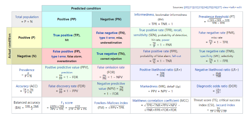
首先是混淆矩阵以及由混下矩阵计算的各种指标:
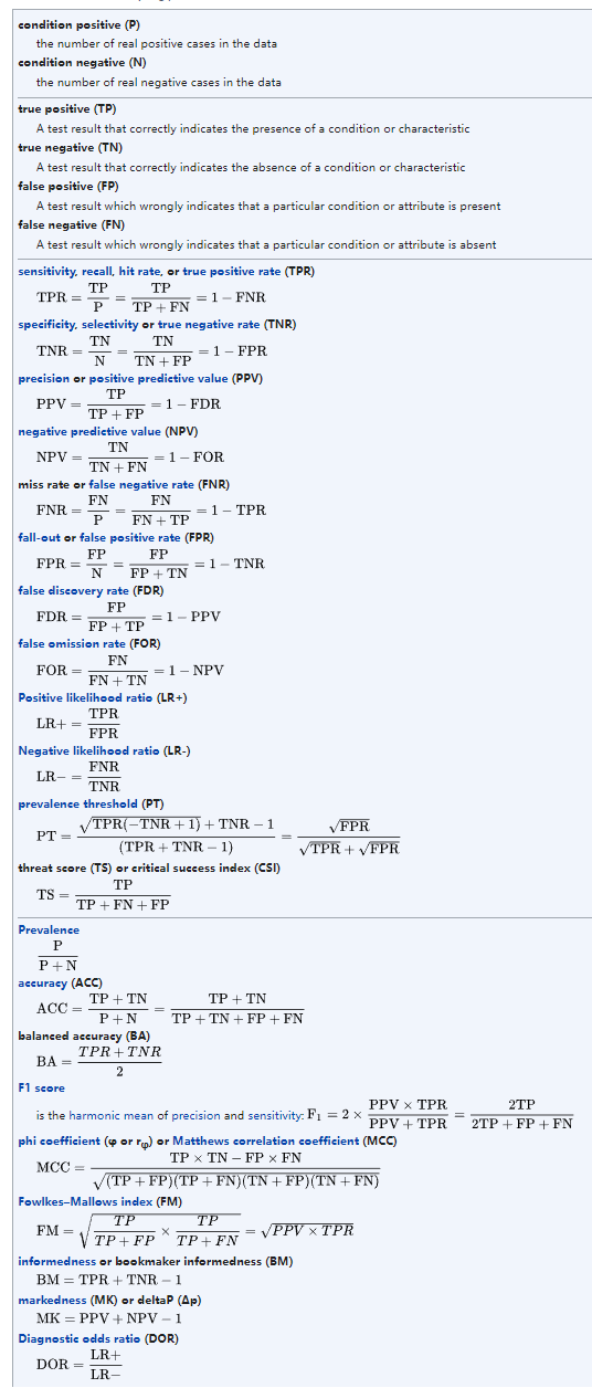
然后是各种常见指标的计算方法:
R语言中有非常多的方法可以实现ROC曲线,但是基本上都是至少需要2列数据,一列是真实结果,另一列是预测值,有了这两列数据,就可以轻松使用各种方法画出ROC曲线并计算AUC。
这篇文章带大家介绍最常见的并且好用的二分类变量的ROC曲线画法。
24.1 方法1:pROC
使用pROC包,不过使用这个包需要注意,一定要指定direction,否则可能会得出错误的结果。
这个R包计算AUC是基于中位数的,哪一组的中位数大就计算哪一组的AUC,在计算时千万要注意!
关于这个R包的详细使用,请参考文章:用pROC实现ROC曲线分析
使用pROC包的aSAH数据,其中outcome列是结果变量,1代表Good,2代表Poor。
计算AUC及可信区间:
res <- roc(aSAH$outcome,aSAH$s100b,ci=T,auc=T)
## Setting levels: control = Good, case = Poor
## Setting direction: controls < cases
res
##
## Call:
## roc.default(response = aSAH$outcome, predictor = aSAH$s100b,     auc = T, ci = T)
##
## Data: aSAH$s100b in 72 controls (aSAH$outcome Good) < 41 cases (aSAH$outcome Poor).
## Area under the curve: 0.7314
## 95% CI: 0.6301-0.8326 (DeLong)plot(res,legacy.axes = TRUE)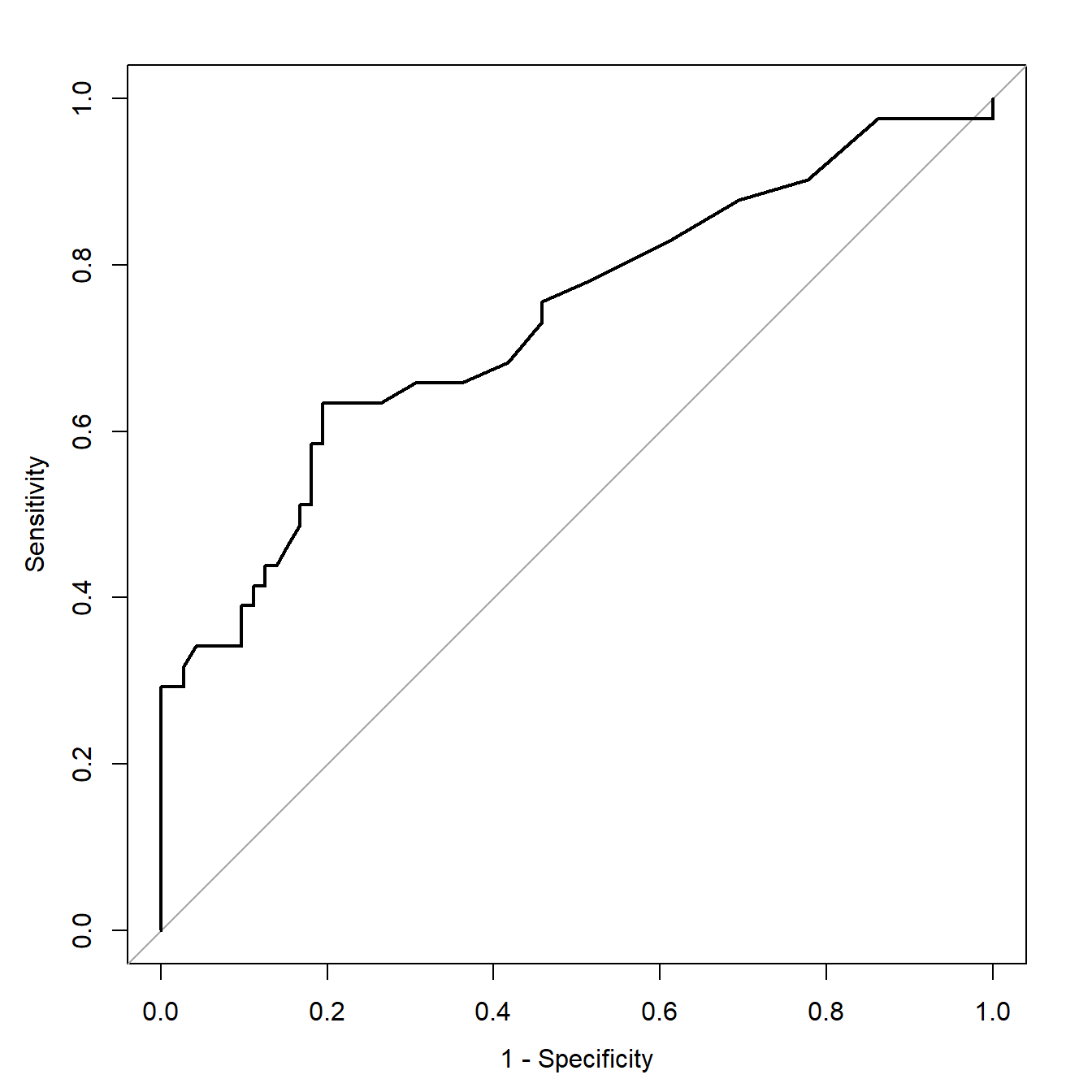
可以显示最佳截点,比如AUC最大的点:
plot(res,
     legacy.axes = TRUE,
     thresholds="best", # AUC最大的点
print.thres="best") 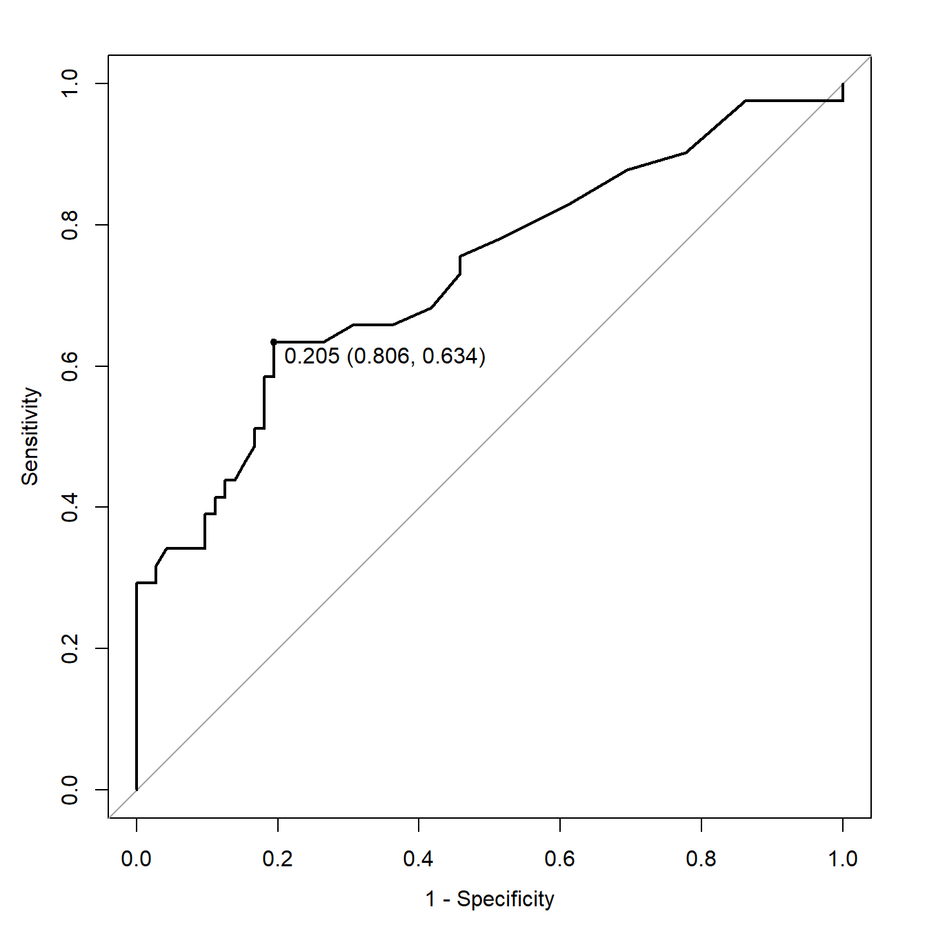
可以显示AUC的可信区间:
rocobj <- plot.roc(aSAH$outcome, aSAH$s100b,
                   main="Confidence intervals",
                   percent=TRUE,ci=TRUE,
                   print.auc=TRUE
                   )
## Setting levels: control = Good, case = Poor
## Setting direction: controls < cases

ciobj <- ci.se(rocobj,
               specificities=seq(0, 100, 5)
               )

plot(ciobj, type="shape", col="#1c61b6AA")
plot(ci(rocobj, of="thresholds", thresholds="best")) 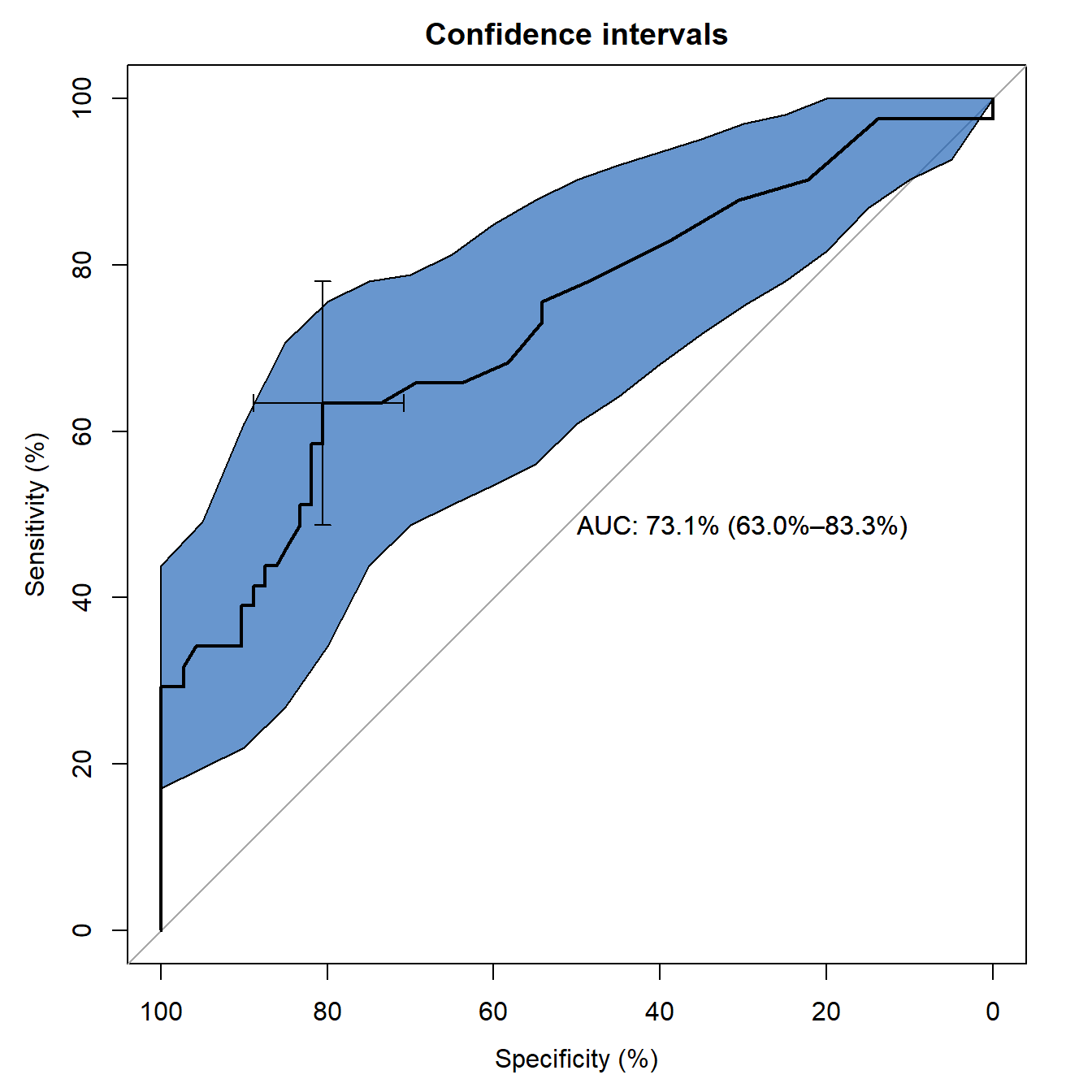
多条ROC曲线画在一起:
rocobj1 <- plot.roc(aSAH$outcome, aSAH$s100,percent=TRUE, col="#1c61b6")
## Setting levels: control = Good, case = Poor
## Setting direction: controls < cases
rocobj2 <- lines.roc(aSAH$outcome, aSAH$ndka, percent=TRUE, col="#008600")
## Setting levels: control = Good, case = Poor
## Setting direction: controls < cases

legend("bottomright", legend=c("S100B", "NDKA"), col=c("#1c61b6", "#008600"), lwd=2)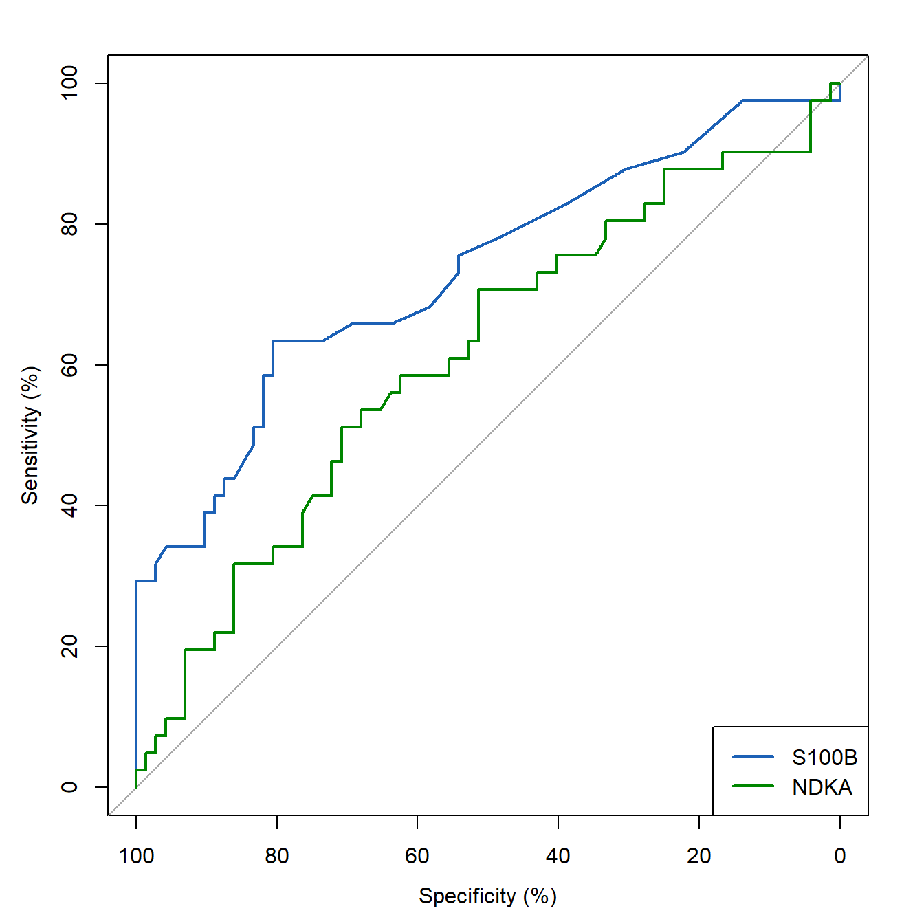
两条ROC曲线的比较,可以添加P值:
rocobj1 <- plot.roc(aSAH$outcome, aSAH$s100,percent=TRUE, col="#1c61b6")
## Setting levels: control = Good, case = Poor
## Setting direction: controls < cases
rocobj2 <- lines.roc(aSAH$outcome, aSAH$ndka, percent=TRUE, col="#008600")
## Setting levels: control = Good, case = Poor
## Setting direction: controls < cases

legend("bottomright", legend=c("S100B", "NDKA"), col=c("#1c61b6", "#008600"), lwd=2)

testobj <- roc.test(rocobj1, rocobj2)

text(50, 50, labels=paste("p-value =", format.pval(testobj$p.value)), adj=c(0, .5))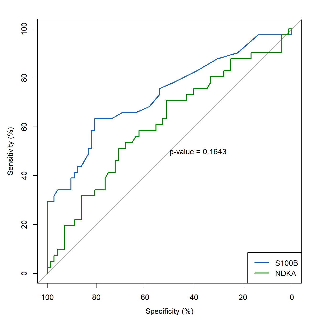
24.2 方法2:ROCR
使用ROCR,如果你只是为了画一条ROC曲线,这是我最推荐的方法了,美观又简单!
library(ROCR)使用非常简单,3句代码,其中第2句是关键,可以更改各种参数,然后就可以画出各种不同的图形:
pred <- prediction(aSAH$s100b,aSAH$outcome)
perf <- performance(pred, "tpr","fpr")
auc <- round(performance(pred, "auc")@y.values[[1]],digits = 4)

plot(perf,lwd=2,col="tomato")
abline(0,1,lty=2)
legend("bottomright", legend="AUC of s100b: 0.7314", col="tomato", lwd=2,bty = "n")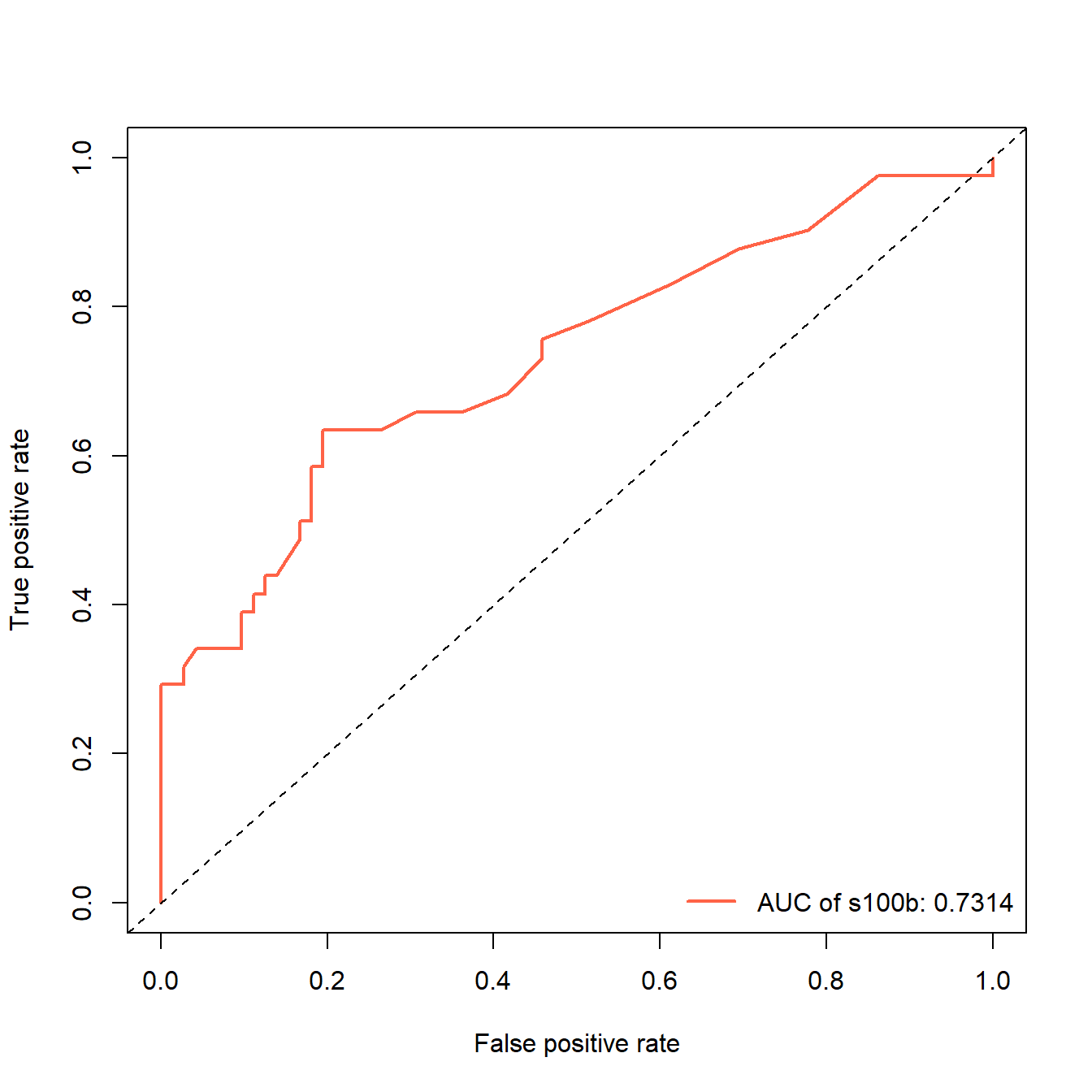
添加箱线图:
perf <- performance(pred, "tpr", "fpr")
perf
## A performance instance
##   'False positive rate' vs. 'True positive rate' (alpha: 'Cutoff')
##   with 51 data points

plot(perf,
     avg="threshold",
     spread.estimate="boxplot")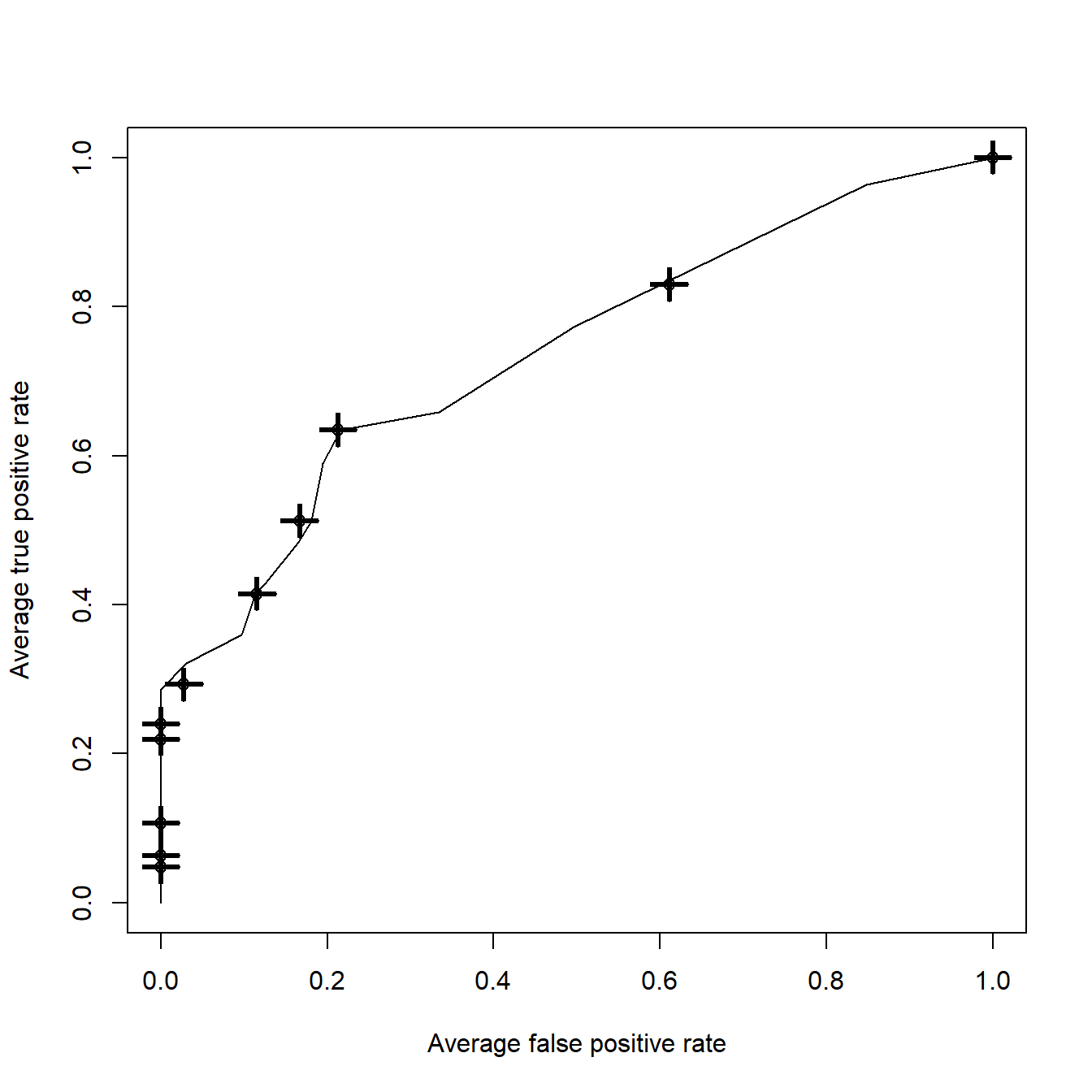
还可以绘制PR曲线,召回率recall为横坐标,精确率precision 为纵坐标:
perf <- performance(pred, "prec", "rec")
plot(perf,
     avg= "threshold",
     colorize=TRUE,
     lwd= 3,
     main= "Precision-Recall plot")
plot(perf,
     lty=3,
     col="grey78",
     add=TRUE)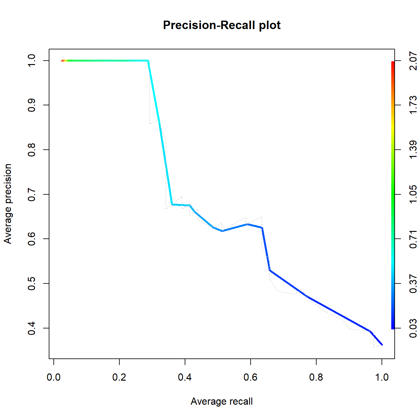
还可以把特异度为横坐标,灵敏度为纵坐标:
perf <- performance(pred, "sens", "spec")
plot(perf,
     avg= "threshold",
     colorize=TRUE,
     lwd= 3,
     main="Sensitivity/Specificity plots")
plot(perf,
     lty=3,
     col="grey78",
     add=TRUE)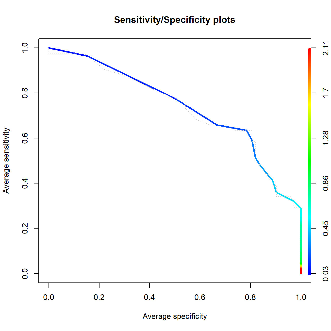
这个包还可以计算非常多其他的指标,各种图都能画,大家可以自己探索。
24.3 方法3:tidymodels
使用tidymodels。这个包很有来头,它是R中专门做机器学习的,可以到公众号:医学和生信笔记中查看更多关于它的教程,它也是目前R语言机器学习领域两大当红辣子鸡之一!另一个是mlr3。
suppressPackageStartupMessages(library(tidymodels))它很优雅,如果你要计算AUC,那么就是roc_auc()函数:
aSAH %>% roc_auc(outcome, s100b,event_level="second")
## # A tibble: 1 × 3
##   .metric .estimator .estimate
##   <chr>   <chr>          <dbl>
## 1 roc_auc binary 0.731如果你是要画ROC曲线,那么就是roc_curve()函数:
aSAH %>% roc_curve(outcome, s100b,event_level="second") %>%
  ggplot(aes(x = 1 - specificity, y = sensitivity)) +
  geom_path(size=1.2,color="firebrick") +
  geom_abline(lty = 3) +
  coord_equal() +
  theme_bw()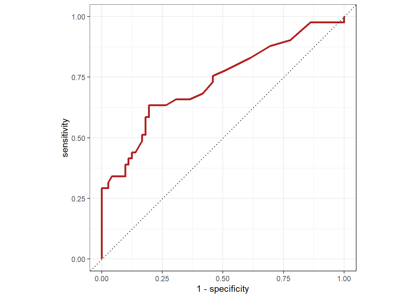
还有太多方法可以画ROC了,不过pROC和ROCR基本上技能解决99%的问题了。
最后,给大家看看cran中比较常见的画ROC曲线的包,大家有兴趣可以自己探索:
library(pkgsearch)

rocPkg <-  pkg_search(query="ROC",size=200)

rocPkgShort <- rocPkg %>%
               filter(maintainer_name != "ORPHANED") %>%
               select(score, package, downloads_last_month) %>%
               arrange(desc(downloads_last_month))
head(rocPkgShort,20)
## # A data frame: 20 × 3
##      score package         downloads_last_month
##  *   <dbl> <chr>                          <int>
##  1 12277.  pROC                          193252
##  2  4486.  caTools                        95766
##  3   974.  ROCR                           48643
##  4   407.  riskRegression                 12488
##  5  2630.  PRROC                           9574
##  6  2291.  cvAUC                           3439
##  7  1829.  plotROC                         3382
##  8   345.  mlr3viz                         2944
##  9  1871.  survivalROC                     2542
## 10   383.  PresenceAbsence                 2474
## 11  1800.  precrec                         2316
## 12  1783.  timeROC                         2287
## 13   115.  RcmdrPlugin.EZR                 2206
## 14   178.  WVPlots                         2021
## 15   466.  ROCit                           1749
## 16   210.  logcondens                      1637
## 17   152.  PredictABEL                     1156
## 18    51.3 wrProteo                         925
## 19   151.  MLeval                           855
## 20 165. cubfits 622pROC高居榜首,遥遥领先!