36  适用一切模型的决策曲线

前面介绍了超多DCA的实现方法，基本上常见的方法都包括了，代码和数据获取方法也给了大家。

今天介绍的是如何实现其他模型的DCA，比如lasso回归、随机森林、决策树、SVM、xgboost等。

这是基于dca.r/stdca.r实现的一种通用方法，使用这个网站给出的代码文件绘制DCA，需要代码的直接去网站下载即可。

注意

这个网站已经不再提供该代码的下载，我很早之前就下载过了，所以我把dca.r/stdca.r这两段代码放在粉丝QQ群文件，需要的加群下载即可（免费的，别问我怎么加群）。

但是原网站下载的stdca.r脚本在某些数据中会遇到以下报错：Error in findrow(fit,times,extend):no points selected for one or more curves, consider using the extend argument，所以我对这段脚本进行了修改，可以解决这个报错，也只能解决这个报错。但是需要付费获取，获取链接：适用于一切模型的DCA，没有任何答疑服务，介意勿扰。

36.1 多个时间点多个cox模型的数据提取

其实ggDCA包完全可以做到，只要1行代码就搞定了，而且功能还很丰富。

我给大家演示一遍基于stdca.r的方法，给大家开阔思路，代码可能不够简洁，但是思路没问题，无非就是各种数据整理与转换。

而且很定会有人对默认结果不满意，想要各种修改，下面介绍的这个方法非常适合自己进行各种自定义！

rm(list = ls())
library(survival)
library(dcurves)
data("df_surv")

# 加载函数
# 原函数有问题，这个是我修改过的
# 获取方式：https://mp.weixin.qq.com/s/TZ7MSaPZZ0Pwomyp_7wqFw
source("E:/R/r-clinical-model/000files/stdca.R") # 原函数有问题

# 构建一个多元cox回归
df_surv$cancer <- as.numeric(df_surv$cancer) # stdca函数需要结果变量是0,1
df_surv <- as.data.frame(df_surv) # stdca函数只接受data.frame

建立多个模型，计算每个模型在不同时间点的概率：

# 建立多个模型
cox_fit1 <- coxph(Surv(ttcancer, cancer) ~ famhistory+marker, 
                  data = df_surv)
cox_fit2 <- coxph(Surv(ttcancer, cancer) ~ age + famhistory + marker, 
                  data = df_surv)
cox_fit3 <- coxph(Surv(ttcancer, cancer) ~ age + famhistory, 
                  data = df_surv)

# 计算每个模型在不同时间点的死亡概率
df_surv$prob11 <- c(1-(summary(survfit(cox_fit1, newdata=df_surv), 
                               times=1)$surv))
df_surv$prob21 <- c(1-(summary(survfit(cox_fit2, newdata=df_surv), 
                               times=1)$surv))
df_surv$prob31 <- c(1-(summary(survfit(cox_fit3, newdata=df_surv), 
                               times=1)$surv))

df_surv$prob12 <- c(1-(summary(survfit(cox_fit1, newdata=df_surv), 
                               times=2)$surv))
df_surv$prob22 <- c(1-(summary(survfit(cox_fit2, newdata=df_surv), 
                               times=2)$surv))
df_surv$prob32 <- c(1-(summary(survfit(cox_fit3, newdata=df_surv), 
                               times=2)$surv))

df_surv$prob13 <- c(1-(summary(survfit(cox_fit1, newdata=df_surv), 
                               times=3)$surv))
df_surv$prob23 <- c(1-(summary(survfit(cox_fit2, newdata=df_surv), 
                               times=3)$surv))
df_surv$prob33 <- c(1-(summary(survfit(cox_fit3, newdata=df_surv), 
                               times=3)$surv))

计算threshold和net benefit：

cox_dca1 <- stdca(data = df_surv, 
      outcome = "cancer", 
      ttoutcome = "ttcancer", 
      timepoint = 1, 
      predictors = c("prob11","prob21","prob31"),
      smooth=TRUE,
      graph = FALSE
    )
## [1] "prob31: No observations with risk greater than 99%, and therefore net benefit not calculable in this range."

cox_dca2 <- stdca(data = df_surv, 
      outcome = "cancer", 
      ttoutcome = "ttcancer", 
      timepoint = 2, 
      predictors = c("prob12","prob22","prob32"),
      smooth=TRUE,
      graph = FALSE
    )

cox_dca3 <- stdca(data = df_surv, 
      outcome = "cancer", 
      ttoutcome = "ttcancer", 
      timepoint = 3, 
      predictors = c("prob13","prob23","prob33"),
      smooth=TRUE,
      graph = FALSE
    )


library(tidyr)
library(dplyr)

36.1.1 第一种数据整理方法

cox_dca_df1 <- cox_dca1$net.benefit
cox_dca_df2 <- cox_dca2$net.benefit
cox_dca_df3 <- cox_dca3$net.benefit

names(cox_dca_df1)[2] <- "all1"
names(cox_dca_df2)[2] <- "all2"
names(cox_dca_df3)[2] <- "all3"

tmp <- cox_dca_df1 %>% 
  left_join(cox_dca_df2) %>% 
  left_join(cox_dca_df3) %>% 
  pivot_longer(cols = contains(c("all","sm","none")),
               names_to = "models",
               values_to = "net_benefit"
               )

画图：

library(ggplot2)
library(ggsci)

ggplot(tmp, aes(x=threshold,y=net_benefit))+
  geom_line(aes(color=models),linewidth=1.2)+
  scale_x_continuous(labels = scales::label_percent(accuracy = 1),
                     name="Threshold Probility")+
  scale_y_continuous(limits = c(-0.05,0.3),name="Net Benefit")+
  theme_bw(base_size = 14)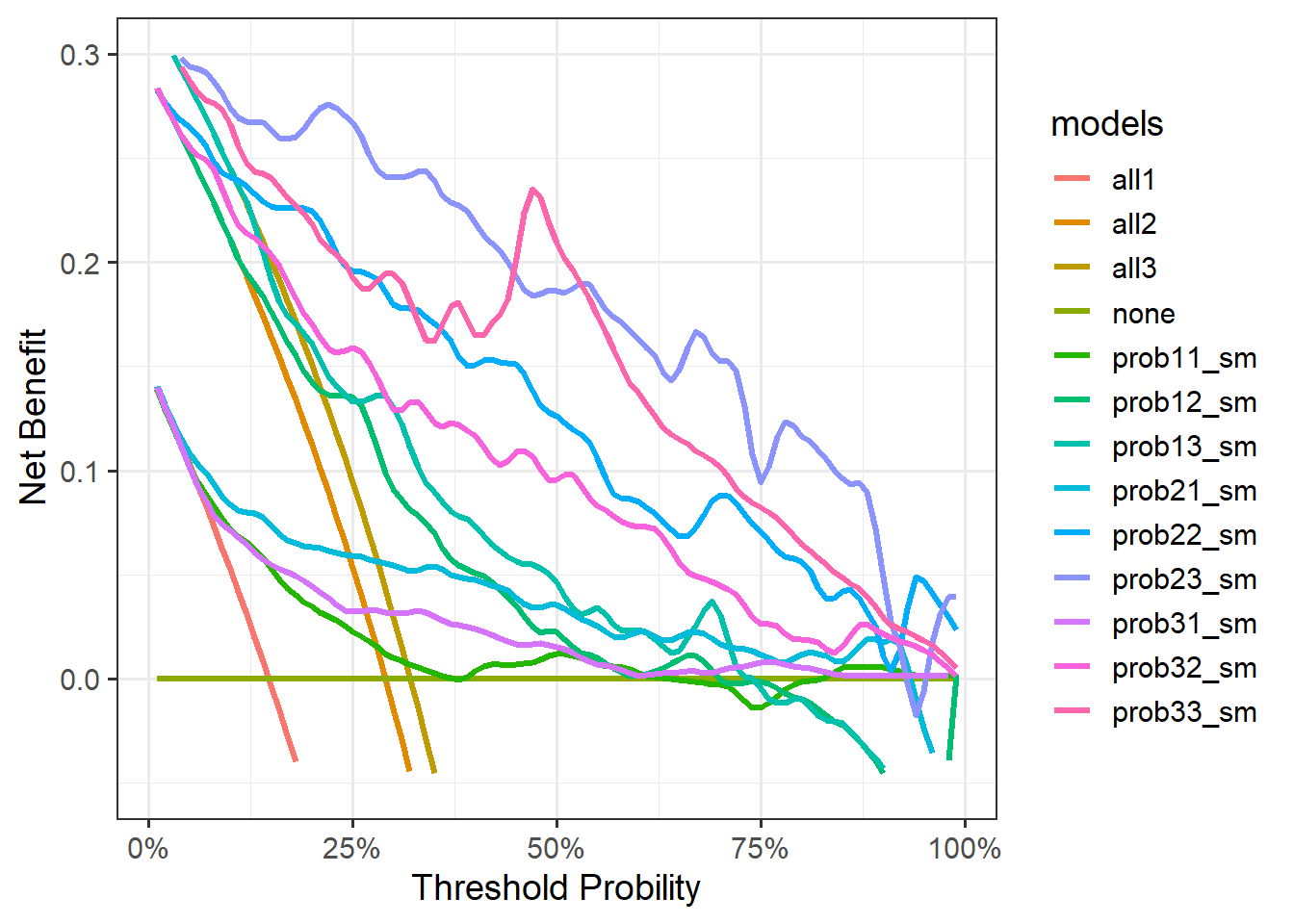

36.1.2 第二种数据整理方法

cox_dca_df1 <- cox_dca1$net.benefit
cox_dca_df2 <- cox_dca2$net.benefit
cox_dca_df3 <- cox_dca3$net.benefit

cox_dca_long_df1 <- cox_dca_df1 %>% 
  rename(mod1 = prob11_sm,
         mod2 = prob21_sm,
         mod3 = prob31_sm
         ) %>% 
  select(-4:-6) %>% 
  mutate(time = "1") %>% 
  pivot_longer(cols = c(all,none,contains("mod")),names_to = "models",
               values_to = "net_benefit"
               )

cox_dca_long_df2 <- cox_dca_df2 %>% 
  rename(mod1 = prob12_sm,
         mod2 = prob22_sm,
         mod3 = prob32_sm
         ) %>% 
  select(-4:-6) %>% 
  mutate(time = "2") %>% 
  pivot_longer(cols = c(all,none,contains("mod")),names_to = "models",
               values_to = "net_benefit"
               )


cox_dca_long_df3 <- cox_dca_df3 %>% 
  rename(mod1 = prob13_sm,
         mod2 = prob23_sm,
         mod3 = prob33_sm
         ) %>% 
  select(-4:-6) %>% 
  mutate(time = "3") %>% 
  pivot_longer(cols = c(all,none,contains("mod")),names_to = "models",
               values_to = "net_benefit"
               )

tes <- bind_rows(cox_dca_long_df1,cox_dca_long_df2,cox_dca_long_df3)

画图：

ggplot(tes,aes(x=threshold,y=net_benefit))+
  geom_line(aes(color=models,linetype=time),linewidth=1.2)+
  scale_x_continuous(labels = scales::label_percent(accuracy = 1),
                     name="Threshold Probility")+
  scale_y_continuous(limits = c(-0.05,0.3),name="Net Benefit")+
  theme_bw(base_size = 14)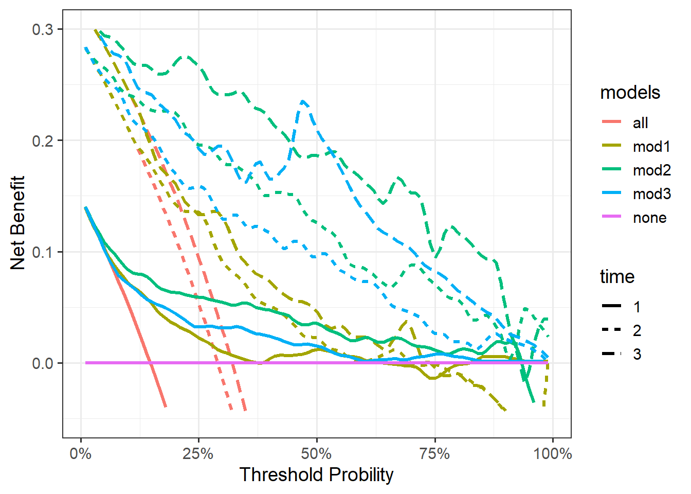

这种方法可以分面。

ggplot(tes,aes(x=threshold,y=net_benefit))+
  geom_line(aes(color=models),linewidth=1.2)+
  scale_y_continuous(limits = c(-0.05,0.3),name="Net Benefit")+
  scale_x_continuous(labels = scales::label_percent(accuracy = 1),
                     name="Threshold Probility")+
  scale_y_continuous(limits = c(-0.05,0.3),name="Net Benefit")+
  theme_bw(base_size = 14)+
  facet_wrap(~time)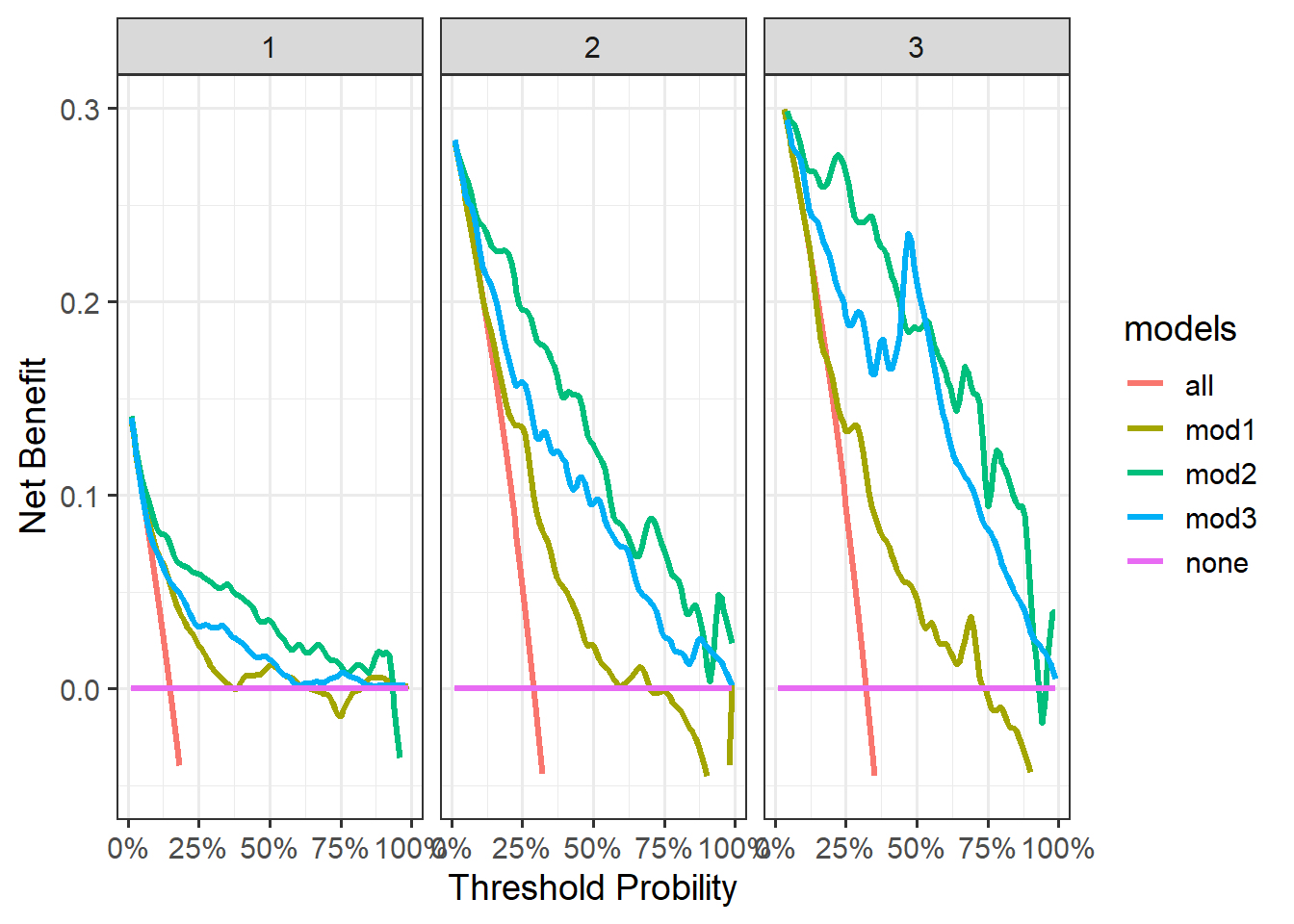

接下来演示其他模型的DCA实现方法，这里就以二分类变量为例，生存资料的DCA也是一样的，就是需要一个概率而已！

36.2 lasso回归

rm(list = ls())
library(glmnet)
library(tidyverse)

准备数据，这是从TCGA下载的一部分数据，其中sample_type是样本类型，1代表tumor，0代表normal，我们首先把因变量变为0,1。然后划分训练集和测试集。

df <- readRDS(file = "./datasets/df_example.rds")

df <- df %>% 
  select(-c(2:3)) %>% 
  mutate(sample_type = ifelse(sample_type=="Tumor",1,0))

set.seed(123)
ind <- sample(1:nrow(df),nrow(df)*0.6)

train_df <- df[ind,]
test_df <- df[-ind,]

构建lasso回归需要的参数值。

x <- as.matrix(train_df[,-1])
y <- train_df$sample_type

在训练集建立lasso回归模型：

cvfit = cv.glmnet(x, y, family = "binomial")
plot(cvfit)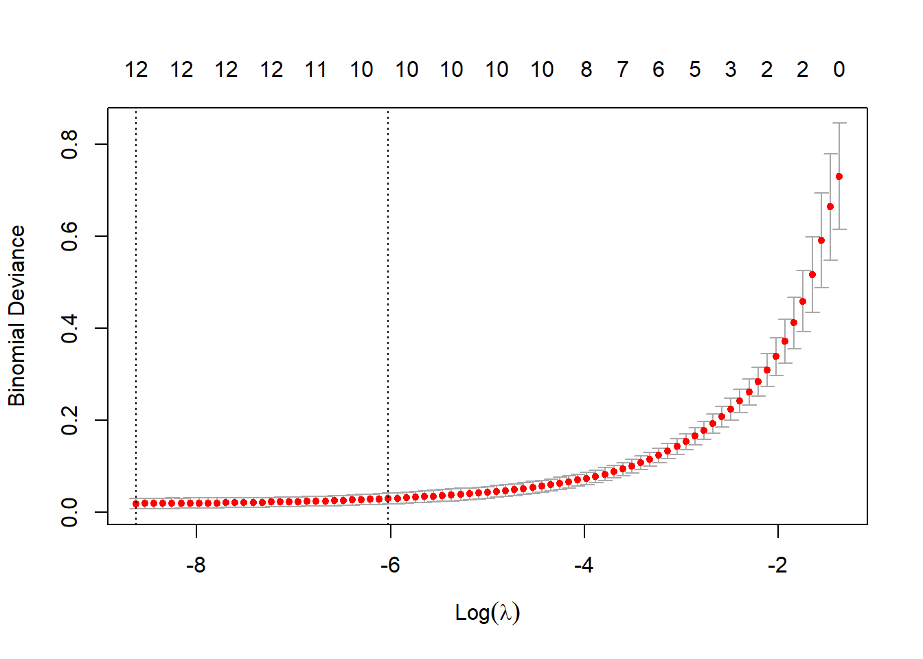

在测试集上查看模型表现：

prob_lasso <- predict(cvfit,
                      newx = as.matrix(test_df[,-1]),
                      s="lambda.1se",
                      type="response") #返回概率

然后进行DCA，也是基于测试集的：

source("./datasets/dca.r")

test_df$lasso <- prob_lasso

df_lasso <- dca(data = test_df, # 指定数据集,必须是data.frame类型
    outcome="sample_type", # 指定结果变量
    predictors="lasso", # 指定预测变量
    probability = T
    )

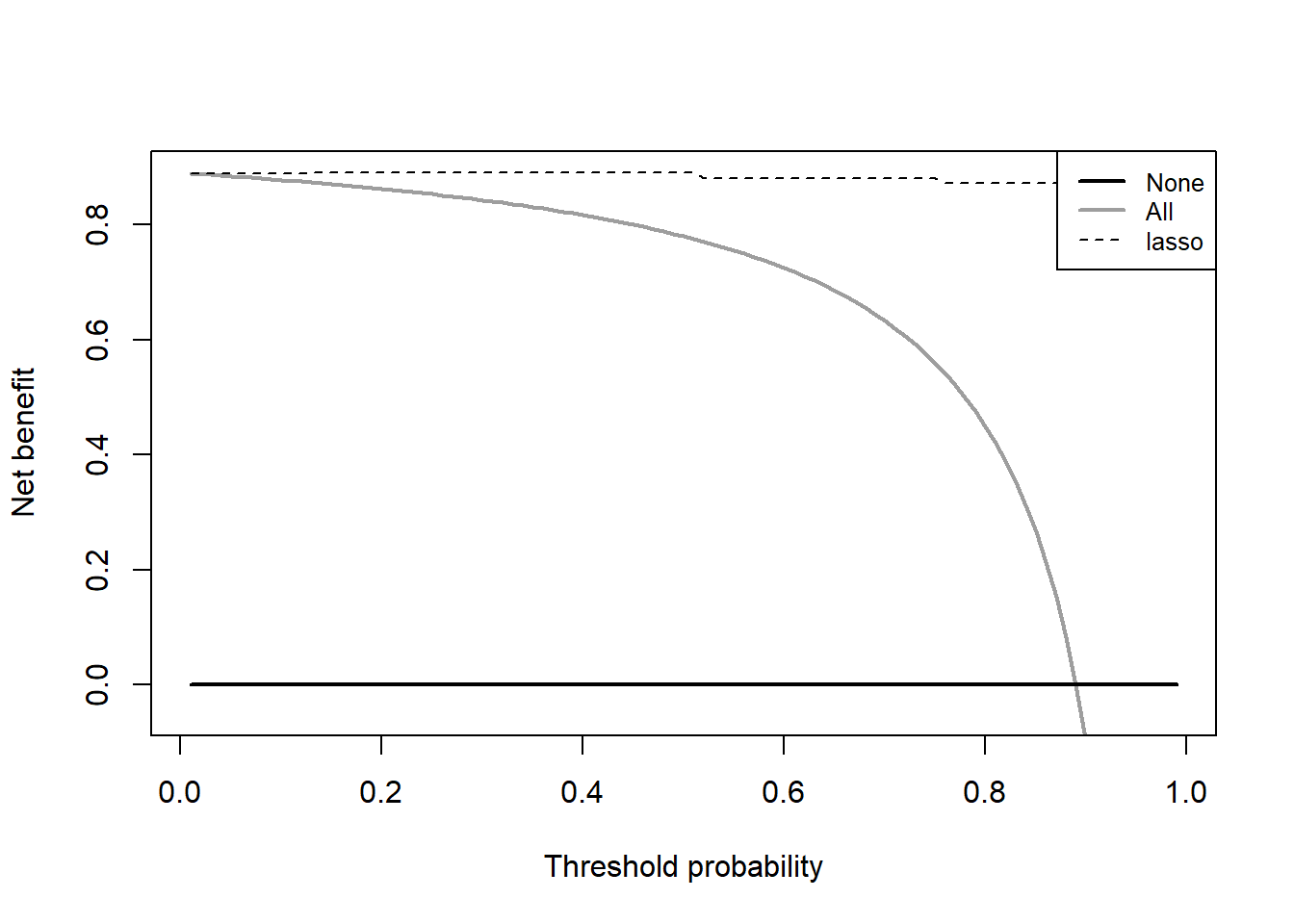
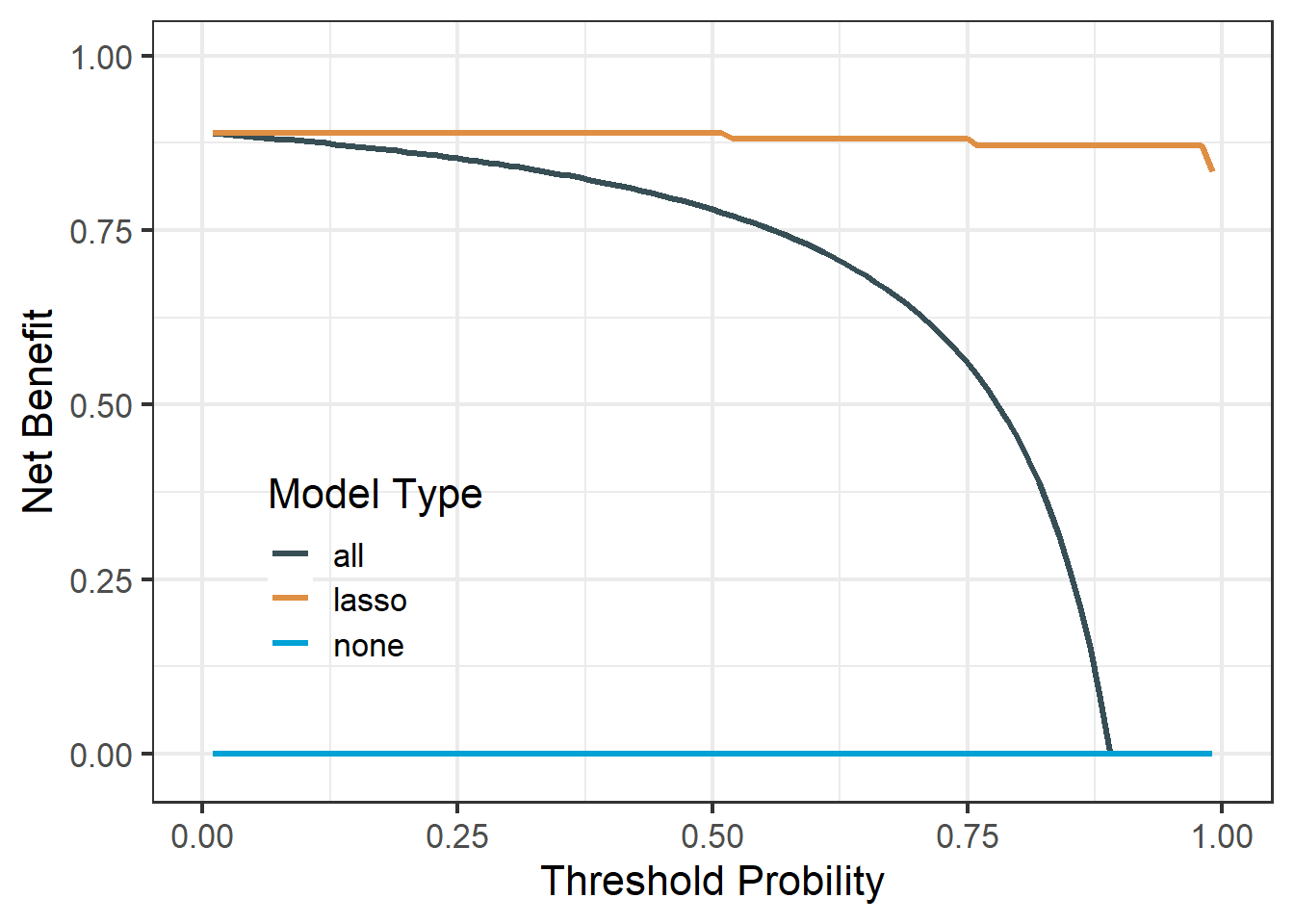
这就是lasso的DCA，由于数据和模型原因，这个DCA看起来很诡异，大家千万要理解实现方法！

library(ggplot2)
library(ggsci)
library(tidyr)

df_lasso$net.benefit %>% 
  pivot_longer(cols = -threshold, 
               names_to = "type", 
               values_to = "net_benefit") %>% 
  ggplot(aes(threshold, net_benefit, color = type))+
  geom_line(linewidth = 1.2)+
  scale_color_jama(name = "Model Type")+ 
  scale_y_continuous(limits = c(-0.02,1),name = "Net Benefit")+ 
  scale_x_continuous(limits = c(0,1),name = "Threshold Probility")+
  theme_bw(base_size = 16)+
  theme(legend.position.inside = c(0.2,0.3),
        legend.background = element_blank()
        )

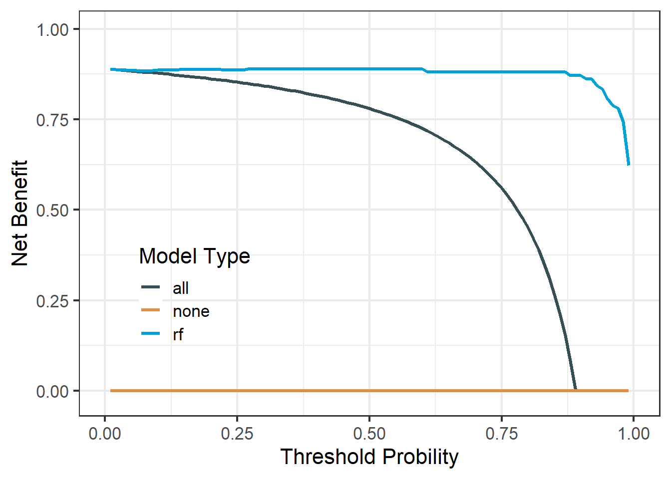
36.3 随机森林

思路完全一样，首先建立随机森林模型，然后计算预测概率（训练集或者测试集都是可以计算的），然后画图即可。

library(ranger)

rf <- ranger(sample_type ~ ., data = train_df)

# 获取测试集的概率
prob_rf <- predict(rf,test_df[,-1],type = "response")$predictions

test_df$rf <- prob_rf

df_rf <- dca(data = test_df, # 指定数据集,必须是data.frame类型
    outcome="sample_type", # 指定结果变量
    predictors="rf", # 指定预测变量
    probability = T,
    graph = F
    )

画图即可：

df_rf$net.benefit %>% 
  pivot_longer(cols = -threshold, 
               names_to = "type", 
               values_to = "net_benefit") %>% 
  ggplot(aes(threshold, net_benefit, color = type))+
  geom_line(linewidth = 1.2)+
  scale_color_jama(name = "Model Type")+ 
  scale_y_continuous(limits = c(-0.02,1),name = "Net Benefit")+ 
  scale_x_continuous(limits = c(0,1),name = "Threshold Probility")+
  theme_bw(base_size = 16)+
  theme(legend.position = c(0.2,0.3),
        legend.background = element_blank()
        )

还有其他比如支持向量机等，就不一一介绍了，实现原理都是一样的，就是需要一个概率而已。

如果是生存分析的话，会比较复杂一点，因为真实概率不好计算，需要指定一个时间点。