# 使用的数据集
library(mlbench)
data(Sonar)

dim(Sonar)
## [1] 208  61
str(Sonar[, 1:10])# 展示前10列
## 'data.frame':    208 obs. of  10 variables:
##  $ V1 : num  0.02 0.0453 0.0262 0.01 0.0762 0.0286 0.0317 0.0519 0.0223 0.0164 ...
##  $ V2 : num  0.0371 0.0523 0.0582 0.0171 0.0666 0.0453 0.0956 0.0548 0.0375 0.0173 ...
##  $ V3 : num  0.0428 0.0843 0.1099 0.0623 0.0481 ...
##  $ V4 : num  0.0207 0.0689 0.1083 0.0205 0.0394 ...
##  $ V5 : num  0.0954 0.1183 0.0974 0.0205 0.059 ...
##  $ V6 : num  0.0986 0.2583 0.228 0.0368 0.0649 ...
##  $ V7 : num  0.154 0.216 0.243 0.11 0.121 ...
##  $ V8 : num  0.16 0.348 0.377 0.128 0.247 ...
##  $ V9 : num  0.3109 0.3337 0.5598 0.0598 0.3564 ...
## $ V10: num 0.211 0.287 0.619 0.126 0.446 ...41 caret实现多模型比较
该方法基于
caret实现,caret曾经是R语言里做机器学习和预测模型最火爆的R包之一(现在不是了),公众号后台回复caret即可获取caret合集链接,带你全面了解caret。
caret是R里面经典的综合性统计建模R包,目前来看已经落后于mlr3和tidymodels了,但是作为老牌R包,日常使用还是没问题的(速度很慢)。
41.1 数据划分
下面是一个分类数据的演示。这个数据一共208行,61列,其中Class是结果变量,二分类,因子型,其余变量都是预测变量。
划分训练集、测试集:
# 加载R包,划分数据集
library(caret)

# 训练集、测试集划分,比例为0.75
set.seed(998)
inTraining <- createDataPartition(Sonar$Class, p = .75, list = FALSE)
training <- Sonar[inTraining,]
testing  <- Sonar[-inTraining,]
41.2 建立多个模型
首先建立一个boosted tree模型,并设置好它的超参数范围以及重抽样方法:
# 网格搜索,首先设定超参数范围
gbmGrid <-  expand.grid(interaction.depth = c(1, 5, 9),
                        n.trees = (1:30)*50,
                        shrinkage = 0.1,
                        n.minobsinnode = 20)

nrow(gbmGrid)
## [1] 90
head(gbmGrid)
##   interaction.depth n.trees shrinkage n.minobsinnode
## 1                 1      50       0.1             20
## 2                 5      50       0.1             20
## 3                 9      50       0.1             20
## 4                 1     100       0.1             20
## 5                 5     100       0.1             20
## 6 9 100 0.1 20设置boosted tree模型的重抽样方法:
# trainControl函数用来设置非常多的东西,重复10次的10折交叉验证
fitControl <- trainControl(method = "repeatedcv",
                           number = 10,
                           repeats = 10,
                           classProbs = TRUE, # 计算概率
                           summaryFunction = twoClassSummary # 二分类指标
                           )
选择好之后开始拟合模型(及超参数调优):
# 选择好之后开始调优
set.seed(825)
gbmFit3 <- train(Class ~ .,
                 data = training,
                 method = "gbm",
                 trControl = fitControl,
                 verbose = FALSE,
                 tuneGrid = gbmGrid,
                 metric = "ROC" # 选择指标
                 )
gbmFit3
#saveRDS(gbmFit3,file = "./datasets/gbmFit3.rds")上面的例子展示了caret包建模的基本语法,就是一个train()就可以了,method参数选择模型,trControl选择重抽样方法,preProcess选择数据预处理方法(上面这个例子没有进行数据预处理)。
train()函数中的metric参数可以指定调优的指标,默认分类模型是accuracy和Kappa,回归模型是RMSE/R2/MAE。
trainControl()中的summaryFunction参数还提供了额外的调优指标选项,比如上面这个twoClassSummary,内含3种指标:敏感度、特异度、ROC。
然后再建立一个支持向量机模型和正则化的判别分析模型。
# 选择重抽样方法,重复10次的10折交叉验证
fitControl <- trainControl(method = "repeatedcv", #默认是simple boost
                           number = 10,
                           repeats = 10,
                           classProbs = T # 计算概率
                           )
开始拟合模型:
# 支持向量机,高斯径向基核
set.seed(825)
svmFit <- train(Class ~ .,
                data = training,
                method = "svmRadial",
                trControl = fitControl,
                preProc = c("center", "scale"),
                tuneLength = 8,
                metric = "ROC")

# 正则化的判别分析
set.seed(825)
rdaFit <- train(Class ~ .,
                data = training,
                method = "rda",
                trControl = fitControl,
                tuneLength = 4,
                metric = "ROC")
#save(svmFit, rdaFit,file = "./datasets/svm_rda_fit.rdata")
这样我们就建立好了3个模型。
41.3 结果查看
可以单独查看每个模型的结果,直击打印即可:
# 比如查看gbm模型
gbmFit3

Stochastic Gradient Boosting

157 samples
 60 predictor
  2 classes: 'M', 'R'

No pre-processing
Resampling: Cross-Validated (10 fold, repeated 10 times)
Summary of sample sizes: 141, 142, 141, 142, 141, 142, ...
Resampling results across tuning parameters:

  interaction.depth  n.trees  ROC        Sens       Spec
  1                    50     0.8634003  0.8631944  0.6905357
  1                   100     0.8844097  0.8486111  0.7544643
##省略一部分,太长了
  9                  1500     0.9181721  0.8805556  0.8039286

Tuning parameter 'shrinkage' was held constant at a value of 0.1

Tuning parameter 'n.minobsinnode' was held constant at a value of 20
ROC was used to select the optimal model using the largest value.
The final values used for the model were n.trees =
 1450, interaction.depth = 5, shrinkage = 0.1 and n.minobsinnode = 20.
结果没什么难度,我就不帮大家翻译了。
也可以一起放入resamples()函数里面,可以得到每个模型的指标的统计值,比如ROC的最大值、最小值、均值、中位数等:
resamps <- resamples(list(GBM = gbmFit3,
                          SVM = svmFit,
                          RDA = rdaFit))
#resamps
summary(resamps)
##
## Call:
## summary.resamples(object = resamps)
##
## Models: GBM, SVM, RDA
## Number of resamples: 100
##
## ROC
##          Min.  1st Qu.    Median      Mean   3rd Qu. Max. NA's
## GBM 0.6964286 0.874504 0.9454365 0.9216468 0.9821429    1    0
## SVM 0.7321429 0.905878 0.9464286 0.9339658 0.9821429    1    0
## RDA 0.5625000 0.812500 0.8750000 0.8698115 0.9392361    1    0
##
## Sens
##          Min.   1st Qu.    Median      Mean 3rd Qu. Max. NA's
## GBM 0.5555556 0.7777778 0.8750000 0.8787500       1    1    0
## SVM 0.5000000 0.7777778 0.8888889 0.8730556       1    1    0
## RDA 0.4444444 0.7777778 0.8750000 0.8604167       1    1    0
##
## Spec
##          Min.   1st Qu.    Median      Mean   3rd Qu. Max. NA's
## GBM 0.4285714 0.7142857 0.8571429 0.8119643 1.0000000    1    0
## SVM 0.4285714 0.7142857 0.8571429 0.8205357 0.9062500    1    0
## RDA 0.1428571 0.5714286 0.7142857 0.6941071 0.8571429    1    0
结果就很强!分别给出了3种指标下的每种模型的统计值。
41.4 结果可视化
喜闻乐见的结果可视化也是必不可少的。主要包括以下几种(都是基于lattice的):
- density plots,
- box-whisker plots,
- scatterplot matrices,
- scatterplots
箱线图:
# 设主题
theme1 <- trellis.par.get()
theme1$plot.symbol$col = rgb(.2, .2, .2, .4)
theme1$plot.symbol$pch = 16
theme1$plot.line$col = rgb(1, 0, 0, .7)
theme1$plot.line$lwd <- 2

# 画图,箱线图
trellis.par.set(theme1)
bwplot(resamps, layout = c(3, 1))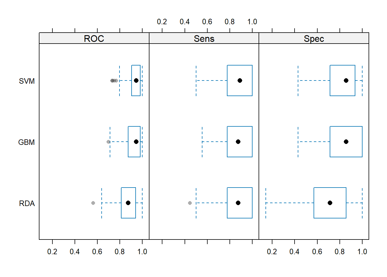
密度图:
# 密度图
trellis.par.set(theme1)
densityplot(resamps)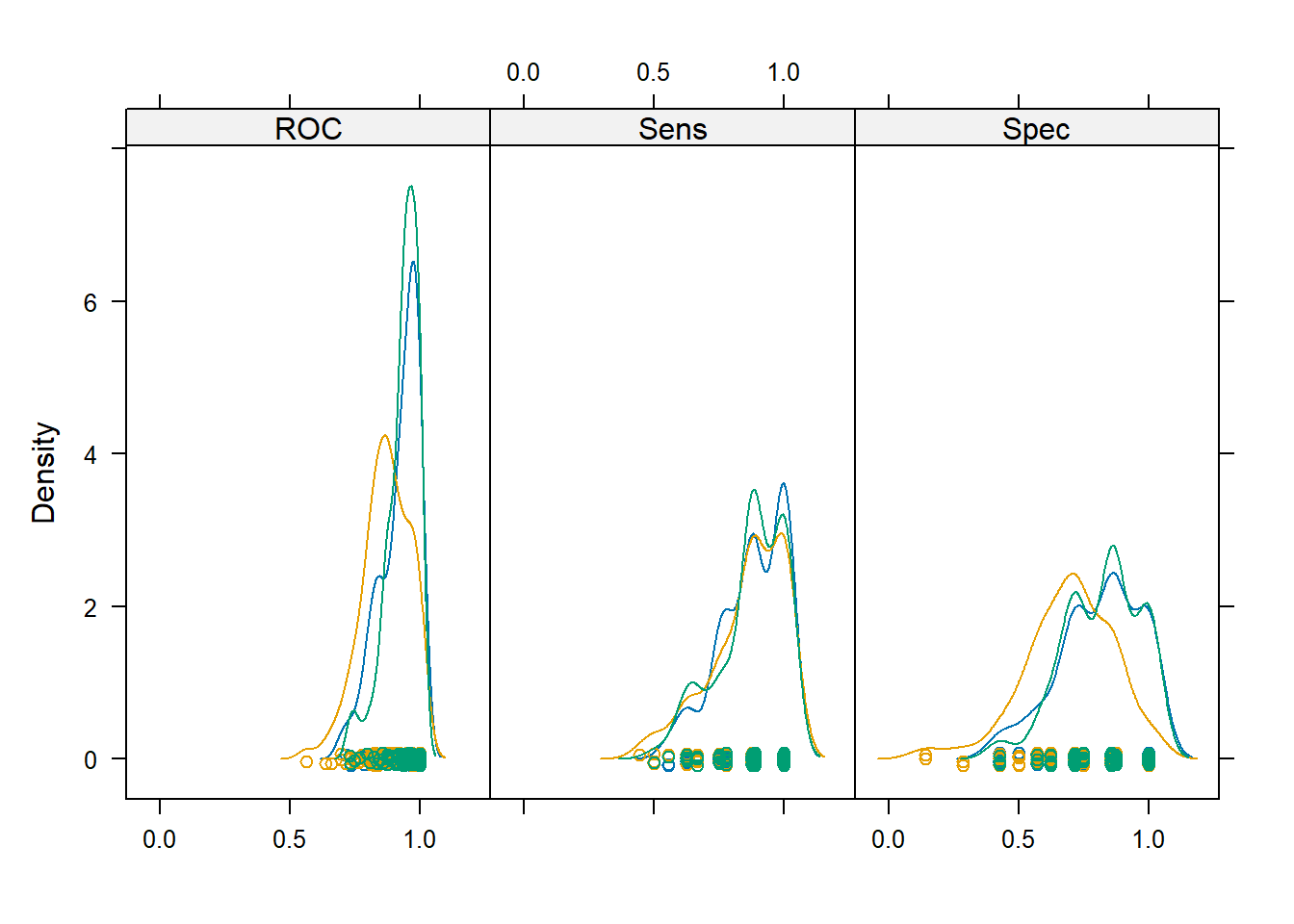
换个指标,点线图:
# 换个指标,点线图
trellis.par.set(caretTheme())
dotplot(resamps, metric = "ROC")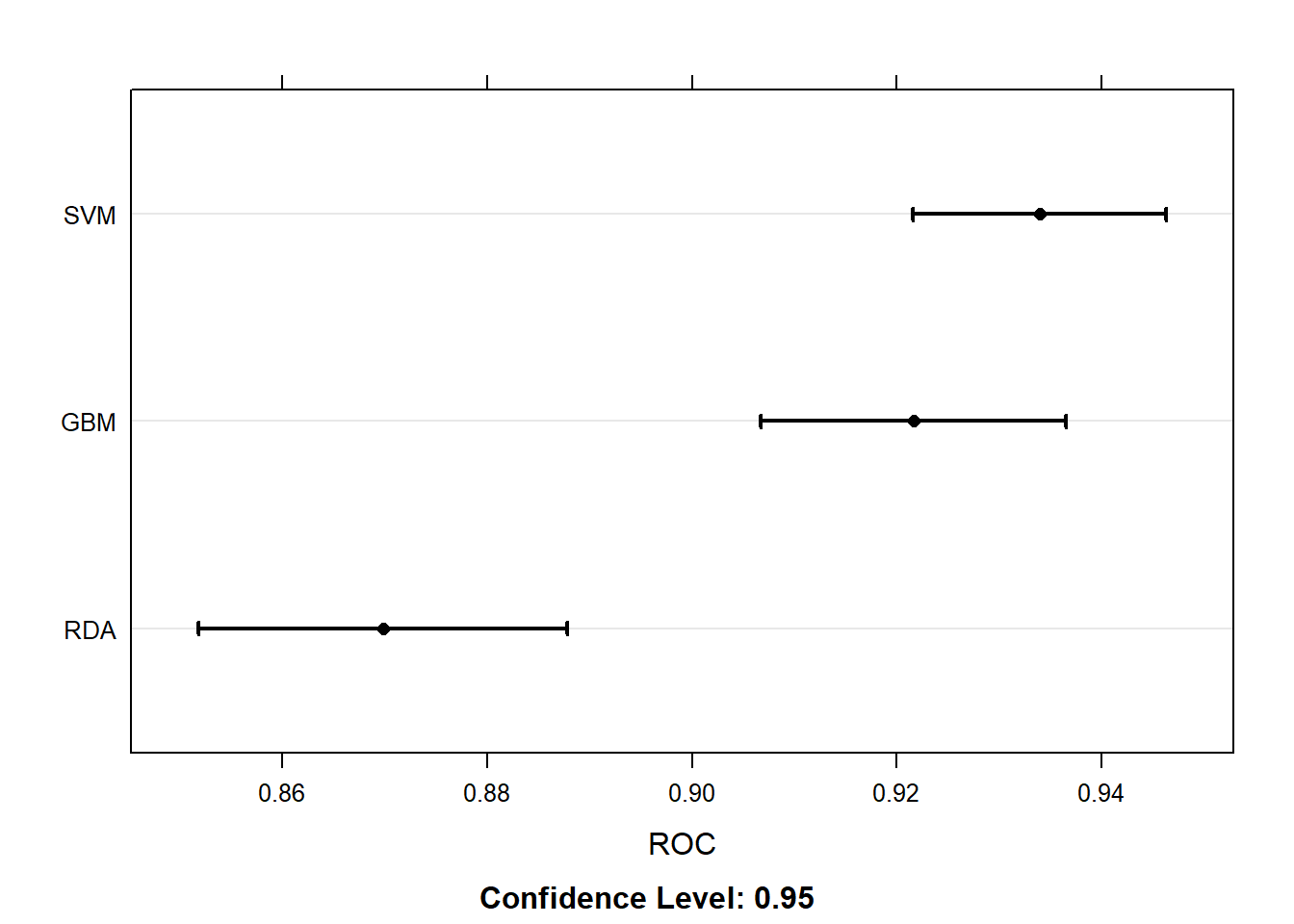
散点图:
# 散点图
trellis.par.set(theme1)
xyplot(resamps, what = "BlandAltman")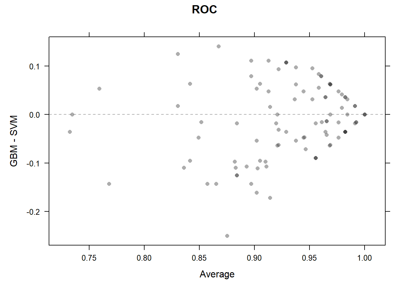
散点图矩阵:
# 散点图矩阵
splom(resamps)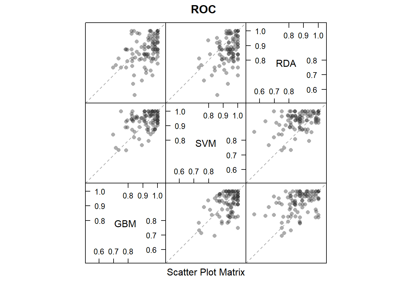
41.5 显著性检验
除此之外,我们还可以对不同模型之间的差异进行显著性检验,比如t检验,结果会给出多重校正检验(bonferroni法)的p值,非常高大上:
difValues <- diff(resamps)
difValues
##
## Call:
## diff.resamples(x = resamps)
##
## Models: GBM, SVM, RDA
## Metrics: ROC, Sens, Spec
## Number of differences: 3
## p-value adjustment: bonferroni
summary(difValues)
##
## Call:
## summary.diff.resamples(object = difValues)
##
## p-value adjustment: bonferroni
## Upper diagonal: estimates of the difference
## Lower diagonal: p-value for H0: difference = 0
##
## ROC
##     GBM       SVM       RDA
## GBM           -0.01232   0.05184
## SVM 0.3408               0.06415
## RDA 5.356e-07 2.638e-10
##
## Sens
##     GBM    SVM      RDA
## GBM        0.005694 0.018333
## SVM 1.0000          0.012639
## RDA 0.4253 1.0000
##
## Spec
##     GBM       SVM       RDA
## GBM           -0.008571  0.117857
## SVM 1                    0.126429
## RDA 8.230e-07 1.921e-10
这个结果展示的是不同模型之间的差异和t检验的p值。比如第一个矩阵(ROC的这个),先横着看,GBM和GBM是一个,不用比,GBM和SVM比,平均ROC的差异是-0.01232,GBM和RDA比,平均ROC的差异是0.05184;再顺着看,GBM和SVM的t检验的p值是0.3408,说明无统计学差异,GBM和RDA的t检验的p值是5.356e-07,有统计学差异。
结果的可视化,使用箱线图,同时展示3种指标,这个图展示的是不同模型之间性能指标的差异分布情况:
trellis.par.set(theme1)
bwplot(difValues, layout = c(3, 1))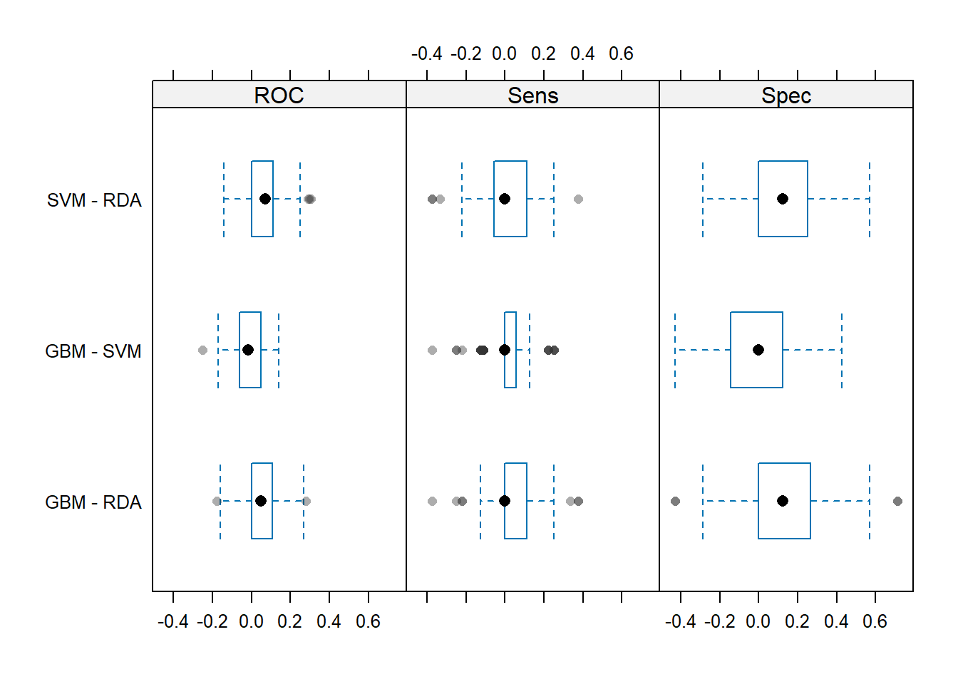
下面这个图展示的是不同模型性能指标差异的95%可信区间,如果通过了0,说明没差异,这个图的结果和上面统计检验的结果是相同的:
trellis.par.set(caretTheme())
dotplot(difValues)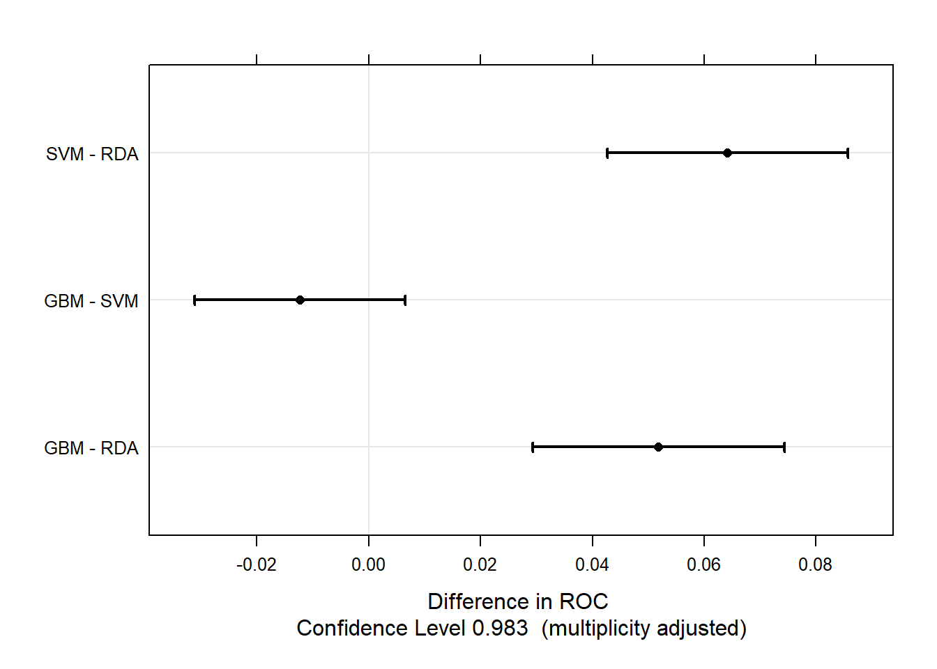
是不是很强!
这里介绍的caret的内容比较简单,大家如果想认真学习这个R包的话肯定是要下一番功夫的,我在公众号写了非常多相关的推文,可以在公众号后台回复caret获取合集。