rm(list = ls())
load(file = "datasets/lnc_expr_clin.RData")
#去掉没有生存信息的样本
lnc_expr_clin1 <- lnc_expr_clin[!is.na(lnc_expr_clin$time_months),]
lnc_expr_clin1 <- lnc_expr_clin1[lnc_expr_clin1$time_months>0,]

#选择其中一部分数据
dat.cox <- lnc_expr_clin1[,c(72:73,1:59)]
dim(dat.cox)
## [1] 297  61
dat.cox[1:4,1:6]
##   event time_months   PGM5-AS1 LINC01082 AC005180.2 AC005180.1
## 1     0       36.33 0.15064007 0.2642238  0.0000000  0.1547768
## 2     0       13.87 0.06309362 0.1666554  0.3105983  0.2436603
## 3     1       21.83 2.16399508 3.5662920  2.2454129  2.0073496
## 4 0 18.20 2.73075081 1.7314314 0.8609916 0.732301415 变量选择之先单后多
先进行单因素分析,有意义的变量继续进行多因素分析,这个可能是大家最先接触到的变量筛选方法,但是这种思路对吗?要不要使用这种方法?
强烈建议大家先阅读冯国双老师的4篇文章,除了能解决以上两个问题外,还解释了为什么单因素有意义多因素却没有意义/单因素无意义多因素有意义的问题:
读完之后看实操~
15.1 准备数据
我们使用TCGA-BLCA的lncRNA数据,其中包括408个样本,time_months是生存时间,event是生存状态,1代表死亡,0代表生存,其余变量都是自变量。
先简单处理一下数据(数据已放在粉丝QQ群文件):
现在这个数据一共59个自变量,我们先对每一个自变量都做一遍单因素COX回归,但是要注意,这里的59个自变量都是连续型的,通常基因表达量增加1,死亡风险增加xx倍这种情况是不可能发生的,这样的结果解释也是不合理的,所以我们需要先把这样的变量重新分箱,比如根据中位数分成两组,再进行单因素COX回归。
dat_cox <- dat.cox
dat_cox[,c(3:ncol(dat_cox))] <- sapply(dat_cox[,c(3:ncol(dat_cox))],function(x){
  ifelse(x>median(x),"high","low")
})
dat_cox[,c(3:ncol(dat_cox))] <- lapply(dat_cox[,c(3:ncol(dat_cox))],factor)
dat_cox[1:4,1:6]
##   event time_months PGM5-AS1 LINC01082 AC005180.2 AC005180.1
## 1     0       36.33     high       low        low        low
## 2     0       13.87      low       low       high       high
## 3     1       21.83     high      high       high       high
## 4     0       18.20     high      high       high       high
15.2 批量单因素cox
然后就可以对每个变量进行单因素COX分析了:
library(survival)

gene <- colnames(dat_cox)[-c(1:2)]
cox.result <- list()
for (i in 1:length(gene)) {
      #print(i)
      group <- dat_cox[, i + 2]
      if (length(table(group)) == 1) next
      #if (length(grep("high", group)) < min_sample_size) next
      #if (length(grep("low", group)) < min_sample_size) next
      x <- survival::coxph(survival::Surv(time_months, event) ~ group,
                           data = dat_cox)
      tmp1 <- broom::tidy(x, exponentiate = T, conf.int = T)
      cox.result[[i]] <- c(gene[i], tmp1)
    }

res.cox <- data.frame(do.call(rbind, cox.result))
筛选出P值小于0.1的变量:
library(dplyr)

unifea <- res.cox %>%
  filter(p.value<0.1) %>%
  pull(V1) %>%
  unlist()
unifea
##  [1] "AC005180.2"   "AC005180.1"   "AC053503.3"   "MIR100HG"     "AP001107.5"
##  [6] "C5orf66-AS1"  "AL162424.1"   "ADAMTS9-AS1"  "MIR200CHG"    "AC093010.3"
## [11] "AC079313.2"   "SNHG25"       "AL049555.1"   "MIR1-1HG-AS1" "SPINT1-AS1"
## [16] "KRT7-AS"      "HAND2-AS1"    "AC025575.2"   "MAFG-DT"      "AL390719.2"
## [21] "AC002398.2"   "AL161431.1"   "U62317.1"     "AL023284.4"   "AATBC"
15.3 多因素cox
把这些变量进行多因素COX回归
sub_dat <- dat_cox[,c("time_months","event",unifea)]
dim(sub_dat)
## [1] 297  27
sub_dat[1:4,1:6]
##   time_months event AC005180.2 AC005180.1 AC053503.3 MIR100HG
## 1       36.33     0        low        low        low      low
## 2       13.87     0       high       high       high      low
## 3       21.83     1       high       high       high     high
## 4       18.20     0       high       high       high     high
拟合多因素cox回归模型并查看结果:
final.fit <- coxph(Surv(time_months,event)~., data = sub_dat)
res <- broom::tidy(final.fit)
res
## # A tibble: 25 × 5
##    term             estimate std.error statistic p.value
##    <chr>               <dbl>     <dbl>     <dbl>   <dbl>
##  1 AC005180.2low      0.146      0.413     0.354 0.723
##  2 AC005180.1low     -0.343      0.399    -0.859 0.390
##  3 AC053503.3low     -0.139      0.391    -0.355 0.723
##  4 MIR100HGlow       -0.365      0.366    -0.997 0.319
##  5 AP001107.5low      0.284      0.344     0.825 0.409
##  6 `C5orf66-AS1`low  -0.538      0.284    -1.89  0.0587
##  7 AL162424.1low      0.0418     0.335     0.125 0.901
##  8 `ADAMTS9-AS1`low  -0.947      0.360    -2.63  0.00853
##  9 MIR200CHGlow       0.0336     0.329     0.102 0.919
## 10 AC093010.3low      0.905      0.323     2.80  0.00505
## # ℹ 15 more rows
查看P值小于0.05的变量:结果只有5个
res %>% filter(p.value<0.05)
## # A tibble: 5 × 5
##   term             estimate std.error statistic p.value
##   <chr>               <dbl>     <dbl>     <dbl>   <dbl>
## 1 `ADAMTS9-AS1`low   -0.947     0.360     -2.63 0.00853
## 2 AC093010.3low       0.905     0.323      2.80 0.00505
## 3 SNHG25low           0.592     0.280      2.11 0.0346
## 4 AC025575.2low       0.618     0.287      2.16 0.0311
## 5 AL161431.1low      -0.704     0.309     -2.28 0.0226
这5个变量可以用于最终的模型中,但是考虑到不同变量之间的交互作用等情况,此时再拟合多因素cox模型,可能还会出现某个变量的P值大于0.05的情况,属于正常现象~
fit5 <- coxph(Surv(time_months,event)~`ADAMTS9-AS1`+AC093010.3+SNHG25+
                AC025575.2+AL161431.1,data = sub_dat)
library(survminer)
survminer::ggforest(fit5)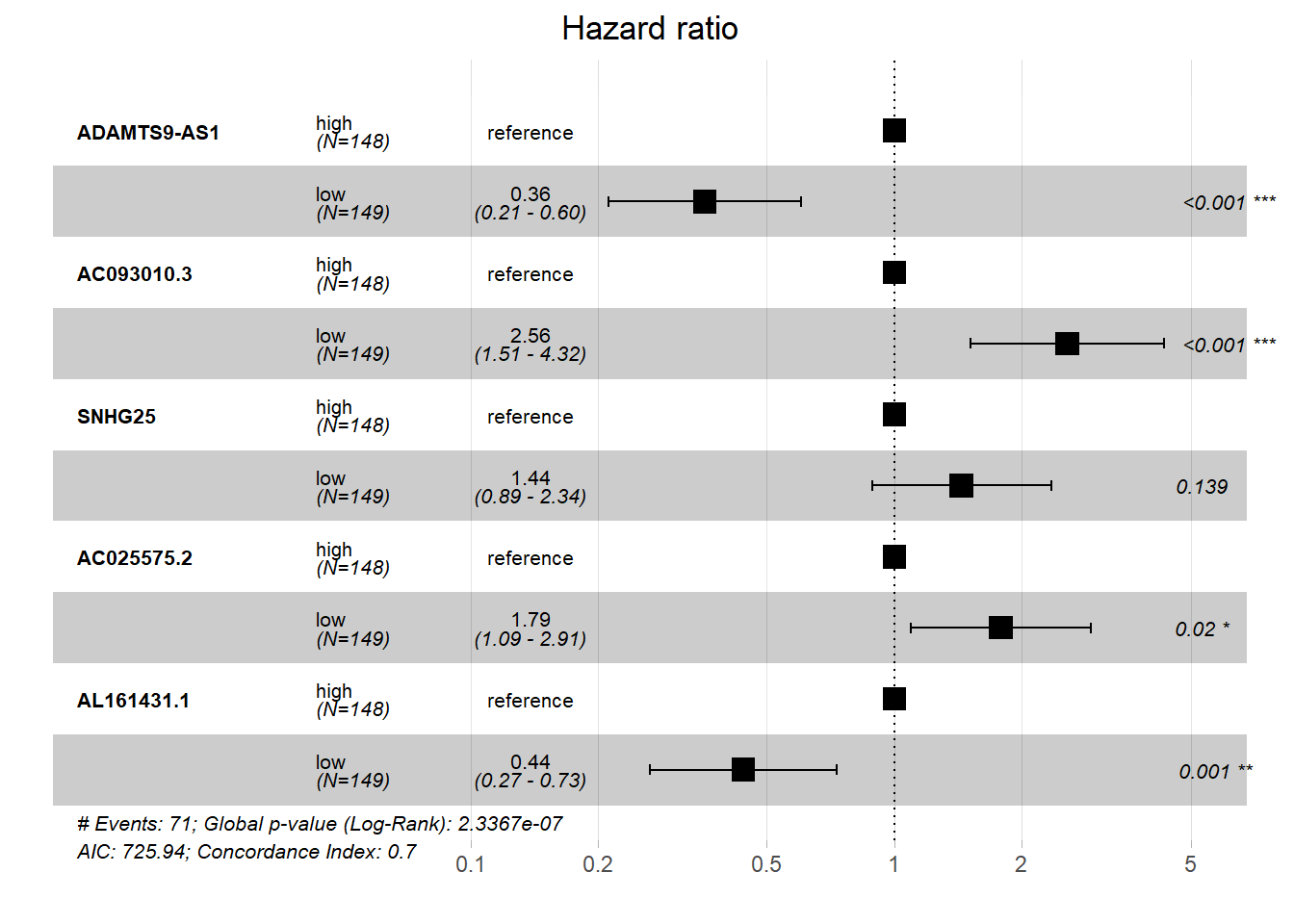
上面这个森林图是多因素回归的森林图,和亚组分析的森林图完全不是一回事,不知道大家有没有注意过呢?
关于森林图和亚组分析的相关问题和详细解释以及各种代码可以在公众号后台回复森林图获取合集。
15.4 1行代码实现
手动实现的过程就是为了告诉大家思路是怎样的,这样大家有一定的基础就可以自己做,不管是什么数据,都是一样的思路,用什么方法和工具不重要,思路才是最重要的。
下面再给大家介绍一个R包,可以实现1行代码完成先单后多cox分析,得到的结果和我们的手动实现的结果是一样的。
首先安装R包:
#install.packages("devtools")
devtools::install_github("cardiomoon/autoReg")library(autoReg)使用autoReg函数可以实现先单后多cox分析,首先先建立cox模型,此时是多因素cox的形式,但是这个函数会自动帮我们提取数据,然后先批量对每个变量做cox。
但是!乱七八糟的变量名字是不行的,比如我们演示用的这个lncRNA数据集,变量名字中有-,导致函数报错:
fit <- coxph(Surv(time_months,event)~., data = dat_cox)

autoReg(fit,
        threshold = 0.1,
        uni = T,
        multi = F
        )

# 报错
Error in parse(text = eq) : <text>:1:23: unexpected symbol
1: df[['MIR1-1HG-AS1']]+1HG
^我们给这个数据集的变量名字修改一下即可,我这里直接把-去掉了:
colnames(dat_cox)<- gsub("-","",colnames(dat_cox))
dat_cox[1:4,1:6]
##   event time_months PGM5AS1 LINC01082 AC005180.2 AC005180.1
## 1     0       36.33    high       low        low        low
## 2     0       13.87     low       low       high       high
## 3     1       21.83    high      high       high       high
## 4     0       18.20    high      high       high       high
这样变量名字中就没有乱七八糟的符号了,此时再进行分析就不会报错了。
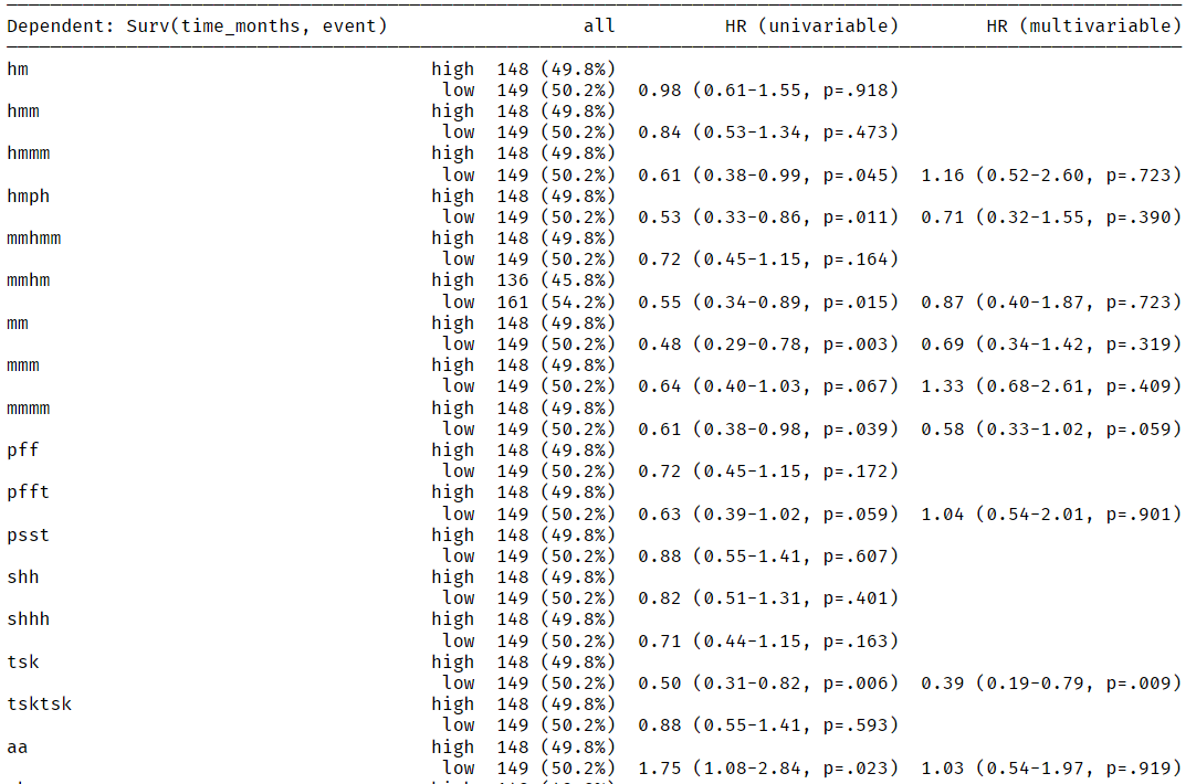
而且结果直接给出了三线表的格式,看起来非常整洁:
fit <- coxph(Surv(time_months,event)~., data = dat_cox)

ft <- autoReg(fit,
        threshold = 0.1,
        uni = T, # 单因素分析
        multi = T, # 多因素分析
        final = F # 逐步法,向后
        )
ft
表格太长了,只展示部分:
这个结果是可以导出为Word或者Excel格式的:
library(rrtable)

table2docx(ft)除此之外,这个包还是一个非常强大的三线表绘制R包,可以1行代码实现多种精美的三线表、回归分析(线性回归、逻辑回归、生存分析)结果表格,大家感兴趣的可以去官网学习:https://cardiomoon.github.io/autoReg/index.html