rm(list = ls())
library(tidyverse)
library(tidymodels)
library(kknn)
tidymodels_prefer()

# 加载数据
all_plays <- read_rds("./datasets/all_plays.rds")
glimpse(all_plays)
## Rows: 91,976
## Columns: 26
## $ game_id                    <dbl> 2017090700, 2017090700, 2017090700, 2017090…
## $ posteam                    <chr> "NE", "NE", "NE", "NE", "NE", "NE", "NE", "…
## $ play_type                  <fct> pass, pass, run, run, pass, run, pass, pass…
## $ yards_gained               <dbl> 0, 8, 8, 3, 19, 5, 16, 0, 2, 7, 0, 3, 10, 0…
## $ ydstogo                    <dbl> 10, 10, 2, 10, 7, 10, 5, 2, 2, 10, 10, 10, …
## $ down                       <ord> 1, 2, 3, 1, 2, 1, 2, 1, 2, 1, 1, 2, 3, 1, 2…
## $ game_seconds_remaining     <dbl> 3595, 3589, 3554, 3532, 3506, 3482, 3455, 3…
## $ yardline_100               <dbl> 73, 73, 65, 57, 54, 35, 30, 2, 2, 75, 32, 3…
## $ qtr                        <ord> 1, 1, 1, 1, 1, 1, 1, 1, 1, 1, 1, 1, 1, 1, 1…
## $ posteam_score              <dbl> 0, 0, 0, 0, 0, 0, 0, 0, 0, 0, 7, 7, 7, 7, 7…
## $ defteam                    <chr> "KC", "KC", "KC", "KC", "KC", "KC", "KC", "…
## $ defteam_score              <dbl> 0, 0, 0, 0, 0, 0, 0, 0, 0, 7, 0, 0, 0, 0, 0…
## $ score_differential         <dbl> 0, 0, 0, 0, 0, 0, 0, 0, 0, -7, 7, 7, 7, 7, …
## $ shotgun                    <fct> 0, 0, 1, 1, 1, 0, 1, 0, 0, 1, 1, 1, 1, 1, 0…
## $ no_huddle                  <fct> 0, 0, 0, 1, 1, 1, 1, 0, 0, 0, 0, 0, 0, 0, 0…
## $ posteam_timeouts_remaining <fct> 3, 3, 3, 3, 3, 3, 3, 3, 3, 3, 3, 3, 3, 3, 3…
## $ defteam_timeouts_remaining <fct> 3, 3, 3, 3, 3, 3, 3, 3, 3, 3, 3, 3, 3, 3, 3…
## $ wp                         <dbl> 0.5060180, 0.4840546, 0.5100098, 0.5529816,…
## $ goal_to_go                 <fct> 0, 0, 0, 0, 0, 0, 0, 1, 1, 0, 0, 0, 0, 0, 0…
## $ half_seconds_remaining     <dbl> 1795, 1789, 1754, 1732, 1706, 1682, 1655, 1…
## $ total_runs                 <dbl> 0, 0, 0, 1, 2, 2, 3, 3, 3, 0, 4, 4, 4, 5, 5…
## $ total_pass                 <dbl> 0, 1, 2, 2, 2, 3, 3, 4, 5, 0, 5, 6, 7, 7, 8…
## $ previous_play              <fct> First play of Drive, pass, pass, run, run, …
## $ in_red_zone                <fct> 0, 0, 0, 0, 0, 0, 0, 1, 1, 0, 0, 0, 0, 1, 1…
## $ in_fg_range                <fct> 0, 0, 0, 0, 0, 1, 1, 1, 1, 0, 1, 1, 1, 1, 1…
## $ two_min_drill <fct> 0, 0, 0, 0, 0, 0, 0, 0, 0, 0, 0, 0, 0, 0, 0…39 tidymodels实现多模型比较
该方法基于
tidymodels实现,tidymodels是目前R语言里做机器学习和预测模型的当红辣子鸡之一(另一个是mlr3),公众号后台回复tidymodels即可获取tidymodels合集链接,带你全面了解tidymodels。另外,我翻译的《tidy modeling with R》中文版-《R语言整洁建模》,也已开卖,感兴趣的朋友不要错过。
在实际操作临床预测模型的建立时,有很多时候我们是要同时建立多个模型的。如果每个模型都写一遍代码,就会非常的费事儿,比如你要建立4个模型,那么就需要把相同的流程写4遍代码,那要是选择10个模型,就得来10遍!无聊,非常的无聊。
所以这里给大家介绍简便方法,不用重复写代码,一次搞定多个模型!使用tidymodels中的workflow即可。
这个”工作流”的概念请参考tidymodels工作流:workflow,这个工具十分强大,下面用一个示例进行展示。
39.1 加载数据和R包
今天用的这份数据,结果变量是一个二分类的。一共有91976行,26列,其中play_type是结果变量,因子型,其余列都是预测变量。
39.2 数据划分
把75%的数据用于训练集,剩下的做测试集。
set.seed(20220520)

# 数据划分,根据play_type分层
split_pbp <- initial_split(all_plays, 0.75, strata = play_type)

train_data <- training(split_pbp) # 训练集
test_data <- testing(split_pbp) # 测试集

dim(train_data)
## [1] 68981    26
dim(test_data)
## [1] 22995    26
39.3 数据预处理
我们对这个数据进行一些简单的预处理:
- 去掉一些没用的变量
- 把一些变量从字符型变成因子型
- 去掉高度相关的变量
- 数值型变量进行中心化
- 去掉零方差变量
pbp_rec <- recipe(play_type ~ ., data = train_data)  %>%
  step_rm(half_seconds_remaining,yards_gained, game_id) %>%
  step_string2factor(posteam, defteam) %>%
  step_corr(all_numeric(), threshold = 0.7) %>%
  step_center(all_numeric()) %>%
  step_zv(all_predictors())
39.4 选择模型
直接选择4个模型,你想选几个都是可以的。
# 逻辑回归模型
lm_mod <- logistic_reg(mode = "classification",engine = "glm")
# K最近邻模型
knn_mod <- nearest_neighbor(mode = "classification", engine = "kknn")
# 随机森林模型
rf_mod <- rand_forest(mode = "classification", engine = "ranger")
# 决策树模型
tree_mod <- decision_tree(mode = "classification",engine = "rpart")
39.5 选择重抽样方法
我们选择内部重抽样方法为10折交叉验证:
set.seed(20220520)

folds <- vfold_cv(train_data, v = 10)
folds
## #  10-fold cross-validation
## # A tibble: 10 × 2
##    splits               id
##    <list>               <chr>
##  1 <split [62082/6899]> Fold01
##  2 <split [62083/6898]> Fold02
##  3 <split [62083/6898]> Fold03
##  4 <split [62083/6898]> Fold04
##  5 <split [62083/6898]> Fold05
##  6 <split [62083/6898]> Fold06
##  7 <split [62083/6898]> Fold07
##  8 <split [62083/6898]> Fold08
##  9 <split [62083/6898]> Fold09
## 10 <split [62083/6898]> Fold10
39.6 构建workflow
这一步就是不用重复写代码的关键,把所有模型和数据预处理步骤自动连接起来。
library(workflowsets)

four_mods <- workflow_set(list(rec = pbp_rec), # 预处理
                          list(lm = lm_mod,    # 模型
                               knn = knn_mod,
                               rf = rf_mod,
                               tree = tree_mod
                               ),
                          cross = T
                          )
four_mods
## # A workflow set/tibble: 4 × 4
##   wflow_id info             option    result
##   <chr>    <list>           <list>    <list>
## 1 rec_lm   <tibble [1 × 4]> <opts[0]> <list [0]>
## 2 rec_knn  <tibble [1 × 4]> <opts[0]> <list [0]>
## 3 rec_rf   <tibble [1 × 4]> <opts[0]> <list [0]>
## 4 rec_tree <tibble [1 × 4]> <opts[0]> <list [0]>
而且你会发现我们虽然设置了预处理步骤,但是并没有进行预处理,展示因为当我们建立工作流之后,它会自动进行这一步,不需要我们提前处理好。这个概念一定要理解。
39.7 同时拟合多个模型
首先是一些运行过程中的参数设置:
# 保存中间的结果
keep_pred <- control_resamples(save_pred = T, verbose = T)
然后就是同时运行4个模型(目前一直是在训练集中),我们给它加速一下:
library(doParallel)

cl <- makePSOCKcluster(12) # 加速,用12个线程
registerDoParallel(cl)

four_fits <- four_mods %>%
  workflow_map("fit_resamples",
               seed = 0520,
               verbose = T,
               resamples = folds,
               control = keep_pred
               )

i 1 of 4 resampling: rec_lm
✔ 1 of 4 resampling: rec_lm (26.6s)
i 2 of 4 resampling: rec_knn
✔ 2 of 4 resampling: rec_knn (3m 44.1s)
i 3 of 4 resampling: rec_rf
✔ 3 of 4 resampling: rec_rf (1m 10.9s)
i 4 of 4 resampling: rec_tree
✔ 4 of 4 resampling: rec_tree (4.5s)

#saveRDS(four_fits,file="datasets/four_fits.rds")
stopCluster(cl)

four_fits
需要很长时间!大家笔记本如果内存不够可能会失败哦,而且运行完之后R会变得非常卡!
39.8 查看结果
查看模型在训练集中的表现(也就是看各种指标):
collect_metrics(four_fits)
## # A tibble: 8 × 9
##   wflow_id .config          preproc model .metric .estimator  mean     n std_err
##   <chr>    <chr>            <chr>   <chr> <chr>   <chr>      <dbl> <int>   <dbl>
## 1 rec_lm   Preprocessor1_M… recipe  logi… accura… binary     0.724    10 1.91e-3
## 2 rec_lm   Preprocessor1_M… recipe  logi… roc_auc binary     0.781    10 1.88e-3
## 3 rec_knn  Preprocessor1_M… recipe  near… accura… binary     0.671    10 7.31e-4
## 4 rec_knn  Preprocessor1_M… recipe  near… roc_auc binary     0.716    10 1.28e-3
## 5 rec_rf   Preprocessor1_M… recipe  rand… accura… binary     0.732    10 1.48e-3
## 6 rec_rf   Preprocessor1_M… recipe  rand… roc_auc binary     0.799    10 1.90e-3
## 7 rec_tree Preprocessor1_M… recipe  deci… accura… binary     0.720    10 1.97e-3
## 8 rec_tree Preprocessor1_M… recipe  deci… roc_auc binary     0.704    10 2.01e-3
结果中给出了每个模型的AUC值和准确率,哪个大就说明哪个好。
查看每一个预测结果,这个就不运行了,毕竟好几万行,太多了。。。
collect_predictions(four_fits)39.9 可视化结果
直接可视化4个模型的结果,感觉比ROC曲线更好看,还给出了可信区间。
这个图可以自己用ggplot2语法修改。
four_fits %>% autoplot(metric = "roc_auc")+theme_bw()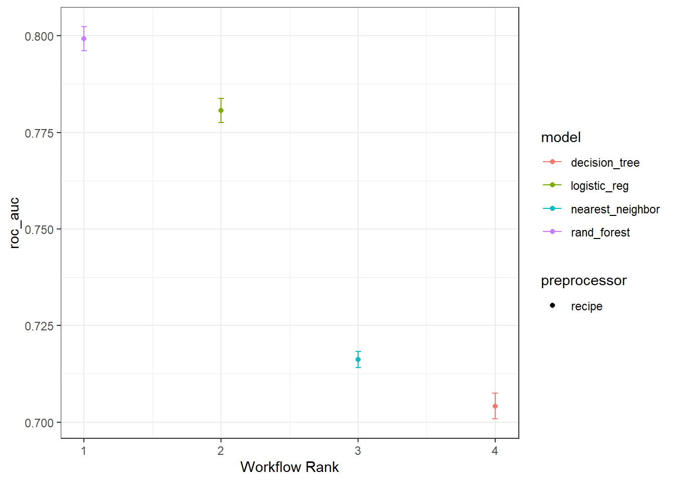
从这个图中来看,随机森林模型是最好的,决策树最差。
39.10 显著性检验
只看大小的话肯定是随机森林最好,但是这种差异有没有统计学意义呢?这就需要专门的统计检验方法了,比如t检验。
在此之前,我们先看看4个模型的AUC之间的相关性如何,也就是计算相关系数:
auc_indiv_estimates <-
  collect_metrics(four_fits, summarize = FALSE) %>%
  filter(.metric == "roc_auc")

auc_wider <-
  auc_indiv_estimates %>%
  select(wflow_id, .estimate, id) %>%
  pivot_wider(id_cols = "id", names_from = "wflow_id", values_from = ".estimate")

corrr::correlate(auc_wider %>% select(-id), quiet = TRUE)
## # A tibble: 4 × 5
##   term     rec_lm rec_knn rec_rf rec_tree
##   <chr>     <dbl>   <dbl>  <dbl>    <dbl>
## 1 rec_lm   NA       0.505  0.933    0.940
## 2 rec_knn   0.505  NA      0.577    0.298
## 3 rec_rf    0.933   0.577 NA        0.860
## 4 rec_tree  0.940   0.298  0.860   NA
上面是一个相关系数矩阵,可以看出线性模型和随机森林以及决策树的AUC相关性很高,随机森林和决策树的AUC相关性也很高,其他模型之间的相关性很低。
下面给大家使用t检验计算一下线性模型和随机森林模型的p值,看看是否有统计学显著性。
# 配对t检验
auc_wider %>%
  with(t.test(rec_lm, rec_rf, paired = TRUE) ) %>%
  tidy() %>%
  select(estimate, p.value, starts_with("conf"))
## # A tibble: 1 × 4
##   estimate  p.value conf.low conf.high
##      <dbl>    <dbl>    <dbl>     <dbl>
## 1  -0.0186 6.74e-10  -0.0202   -0.0170
结果表明p值是小于0.0001的,具有统计学显著性,说明随机森林模型确实比线性回归好。
39.11 选择最好的模型用于测试集
选择表现最好的模型(随机森林)应用于测试集:
rand_res <- last_fit(rf_mod,pbp_rec,split_pbp)
#saveRDS(rand_res,file = "./datasets/rand_res.rds")
查看模型在测试集的模型表现:
collect_metrics(rand_res) # test 中的模型表现
## # A tibble: 2 × 4
##   .metric  .estimator .estimate .config
##   <chr>    <chr>          <dbl> <chr>
## 1 accuracy binary         0.731 Preprocessor1_Model1
## 2 roc_auc  binary         0.799 Preprocessor1_Model1
使用其他指标查看模型表现:
metricsets <- metric_set(accuracy, mcc, f_meas, j_index)

collect_predictions(rand_res) %>%
  metricsets(truth = play_type, estimate = .pred_class)
## # A tibble: 4 × 3
##   .metric  .estimator .estimate
##   <chr>    <chr>          <dbl>
## 1 accuracy binary         0.731
## 2 mcc      binary         0.440
## 3 f_meas   binary         0.774
## 4 j_index  binary         0.438
可视化结果,喜闻乐见的混淆矩阵:
collect_predictions(rand_res) %>%
  conf_mat(play_type,.pred_class) %>%
  autoplot()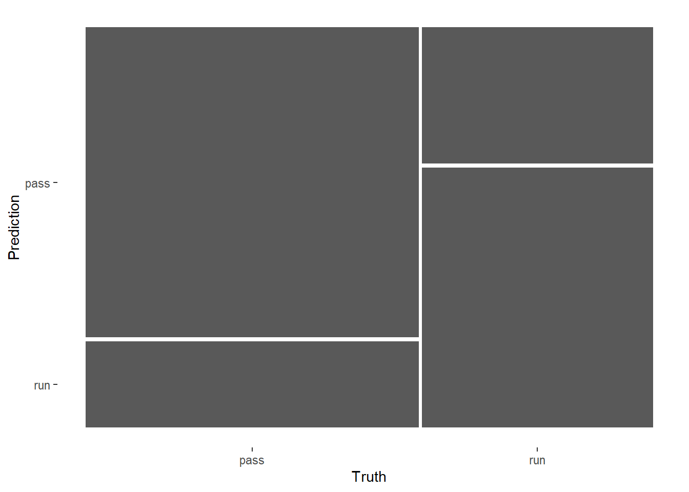
喜闻乐见的ROC曲线:
collect_predictions(rand_res) %>%
  roc_curve(play_type,.pred_pass) %>%
  autoplot()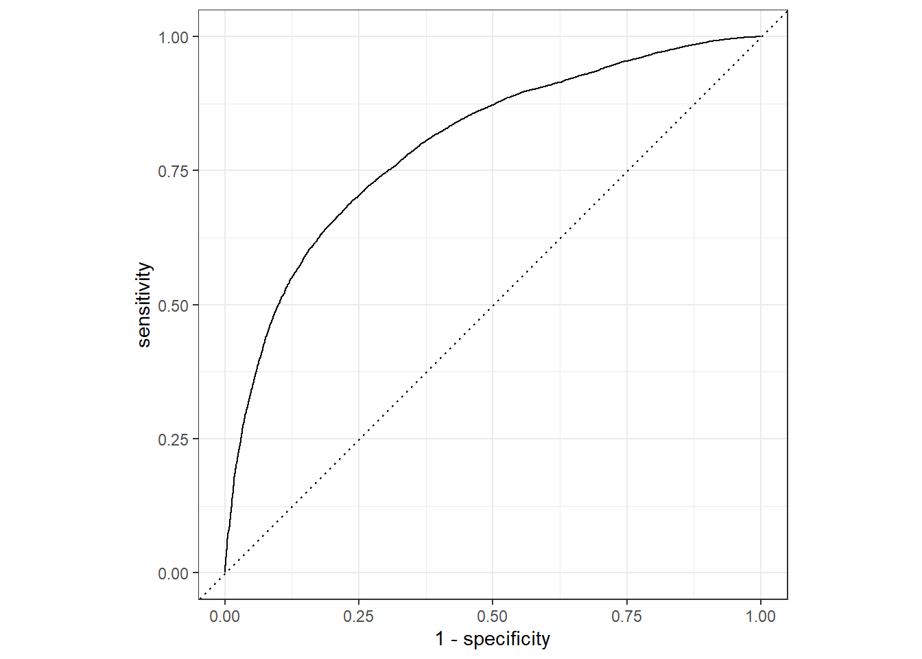
还有非常多曲线和评价指标可选,大家可以看我之前的介绍推文。
这里介绍的tidymodels的内容比较简单,大家如果想认真学习这个R包的话肯定是要下一番功夫的,我在公众号写了非常多相关的推文,可以在公众号后台回复tidymodels获取合集。