rm(list = ls())
suppressPackageStartupMessages(library(tidyverse))
suppressPackageStartupMessages(library(tidymodels))
tidymodels_prefer()46 tidymodels实现多模型比较
注意
这部分内容主要是几个综合性的机器学习和预测建模R包的介绍,更多的信息,可参考机器学习合集
前面介绍了很多二分类资料的模型评价内容,用到了很多R包,虽然达到了目的,但是内容太多了,不太容易记住。
今天给大家介绍很厉害的R包:tidymodels,一个R包搞定二分类资料的模型评价和比较。
一看这个名字就知道,和tidyverse系列师出同门,包的作者是大佬Max Kuhn,大佬的上一个作品是caret,现在加盟rstudio了,开发了新的机器学习R包,也就是今天要介绍的tidymodels。
给大家看看如何用优雅的方式建立、评价、比较多个模型!
46.1 加载数据和R包
没有安装的R包的自己安装下~
由于要做演示用,肯定要一份比较好的数据才能说明问题,今天用的这份数据,结果变量是一个二分类的。
一共有91976行,26列,其中play_type是结果变量,因子型,其余列都是预测变量。
all_plays <- read_rds("./datasets/all_plays.rds")
glimpse(all_plays)
## Rows: 91,976
## Columns: 26
## $ game_id                    <dbl> 2017090700, 2017090700, 2017090700, 2017090…
## $ posteam                    <chr> "NE", "NE", "NE", "NE", "NE", "NE", "NE", "…
## $ play_type                  <fct> pass, pass, run, run, pass, run, pass, pass…
## $ yards_gained               <dbl> 0, 8, 8, 3, 19, 5, 16, 0, 2, 7, 0, 3, 10, 0…
## $ ydstogo                    <dbl> 10, 10, 2, 10, 7, 10, 5, 2, 2, 10, 10, 10, …
## $ down                       <ord> 1, 2, 3, 1, 2, 1, 2, 1, 2, 1, 1, 2, 3, 1, 2…
## $ game_seconds_remaining     <dbl> 3595, 3589, 3554, 3532, 3506, 3482, 3455, 3…
## $ yardline_100               <dbl> 73, 73, 65, 57, 54, 35, 30, 2, 2, 75, 32, 3…
## $ qtr                        <ord> 1, 1, 1, 1, 1, 1, 1, 1, 1, 1, 1, 1, 1, 1, 1…
## $ posteam_score              <dbl> 0, 0, 0, 0, 0, 0, 0, 0, 0, 0, 7, 7, 7, 7, 7…
## $ defteam                    <chr> "KC", "KC", "KC", "KC", "KC", "KC", "KC", "…
## $ defteam_score              <dbl> 0, 0, 0, 0, 0, 0, 0, 0, 0, 7, 0, 0, 0, 0, 0…
## $ score_differential         <dbl> 0, 0, 0, 0, 0, 0, 0, 0, 0, -7, 7, 7, 7, 7, …
## $ shotgun                    <fct> 0, 0, 1, 1, 1, 0, 1, 0, 0, 1, 1, 1, 1, 1, 0…
## $ no_huddle                  <fct> 0, 0, 0, 1, 1, 1, 1, 0, 0, 0, 0, 0, 0, 0, 0…
## $ posteam_timeouts_remaining <fct> 3, 3, 3, 3, 3, 3, 3, 3, 3, 3, 3, 3, 3, 3, 3…
## $ defteam_timeouts_remaining <fct> 3, 3, 3, 3, 3, 3, 3, 3, 3, 3, 3, 3, 3, 3, 3…
## $ wp                         <dbl> 0.5060180, 0.4840546, 0.5100098, 0.5529816,…
## $ goal_to_go                 <fct> 0, 0, 0, 0, 0, 0, 0, 1, 1, 0, 0, 0, 0, 0, 0…
## $ half_seconds_remaining     <dbl> 1795, 1789, 1754, 1732, 1706, 1682, 1655, 1…
## $ total_runs                 <dbl> 0, 0, 0, 1, 2, 2, 3, 3, 3, 0, 4, 4, 4, 5, 5…
## $ total_pass                 <dbl> 0, 1, 2, 2, 2, 3, 3, 4, 5, 0, 5, 6, 7, 7, 8…
## $ previous_play              <fct> First play of Drive, pass, pass, run, run, …
## $ in_red_zone                <fct> 0, 0, 0, 0, 0, 0, 0, 1, 1, 0, 0, 0, 0, 1, 1…
## $ in_fg_range                <fct> 0, 0, 0, 0, 0, 1, 1, 1, 1, 0, 1, 1, 1, 1, 1…
## $ two_min_drill              <fct> 0, 0, 0, 0, 0, 0, 0, 0, 0, 0, 0, 0, 0, 0, 0…
46.2 数据划分
把75%的数据用于训练集,剩下的做测试集。
set.seed(20220520)

# 数据划分,根据play_type分层
split_pbp <- initial_split(all_plays, 0.75, strata = play_type)

train_data <- training(split_pbp) # 训练集
test_data <- testing(split_pbp) # 测试集
46.3 数据预处理
pbp_rec <- recipe(play_type ~ ., data = train_data)  %>%
  step_rm(half_seconds_remaining,yards_gained, game_id) %>% # 移除这3列
  step_string2factor(posteam, defteam) %>%  # 变为因子类型
  #update_role(yards_gained, game_id, new_role = "ID") %>%
  # 去掉高度相关的变量
  step_corr(all_numeric(), threshold = 0.7) %>%
  step_center(all_numeric()) %>%  # 中心化
  step_zv(all_predictors())  # 去掉零方差变量
46.4 建立多个模型
46.4.1 logistic
选择模型,连接数据预处理步骤。
lm_spec <- logistic_reg(mode = "classification",engine = "glm")
lm_wflow <- workflow() %>%
  add_recipe(pbp_rec) %>%
  add_model(lm_spec)
建立模型:
fit_lm <- lm_wflow %>% fit(data = train_data)应用于测试集:
pred_lm <- select(test_data, play_type) %>%
  bind_cols(predict(fit_lm, test_data, type = "prob")) %>%
  bind_cols(predict(fit_lm, test_data))

pred_lm
## # A tibble: 22,995 × 4
##    play_type .pred_pass .pred_run .pred_class
##    <fct>          <dbl>     <dbl> <fct>
##  1 pass           0.399     0.601 run
##  2 pass           0.817     0.183 pass
##  3 pass           0.754     0.246 pass
##  4 pass           0.683     0.317 pass
##  5 run            0.327     0.673 run
##  6 run            0.615     0.385 pass
##  7 pass           0.591     0.409 pass
##  8 run            0.669     0.331 pass
##  9 pass           0.767     0.233 pass
## 10 pass           0.437     0.563 run
## # ℹ 22,985 more rows
查看模型表现:
# 选择多种评价指标
metricsets <- metric_set(accuracy, mcc, f_meas, j_index)

pred_lm %>% metricsets(truth = play_type, estimate = .pred_class)
## # A tibble: 4 × 3
##   .metric  .estimator .estimate
##   <chr>    <chr>          <dbl>
## 1 accuracy binary         0.724
## 2 mcc      binary         0.423
## 3 f_meas   binary         0.774
## 4 j_index  binary         0.416
大家最喜欢的AUC:
pred_lm %>% roc_auc(truth = play_type, .pred_pass)
## # A tibble: 1 × 3
##   .metric .estimator .estimate
##   <chr>   <chr>          <dbl>
## 1 roc_auc binary         0.781
可视化结果,首先是大家喜闻乐见的ROC曲线:
pred_lm %>% roc_curve(truth = play_type, .pred_pass) %>%
  autoplot()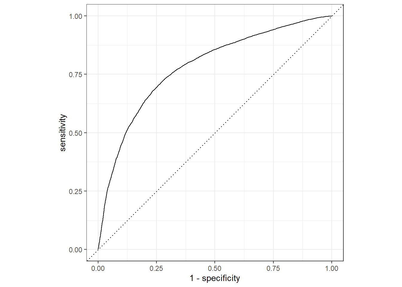
pr曲线:
pred_lm %>% pr_curve(truth = play_type, .pred_pass) %>%
  autoplot()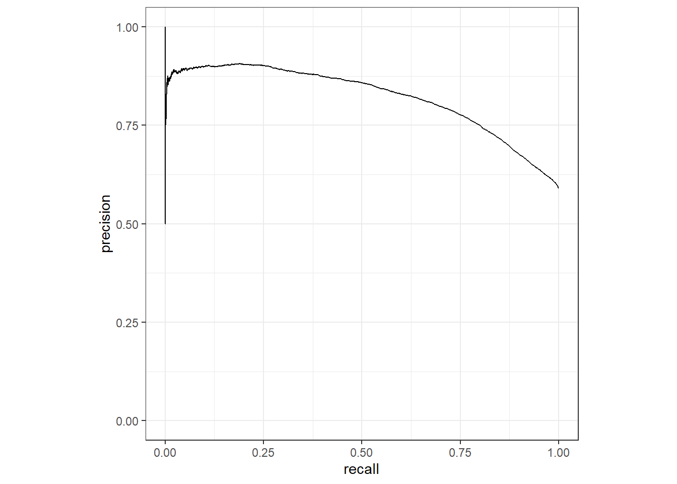
gain_curve:
pred_lm %>% gain_curve(truth = play_type, .pred_pass) %>%
  autoplot()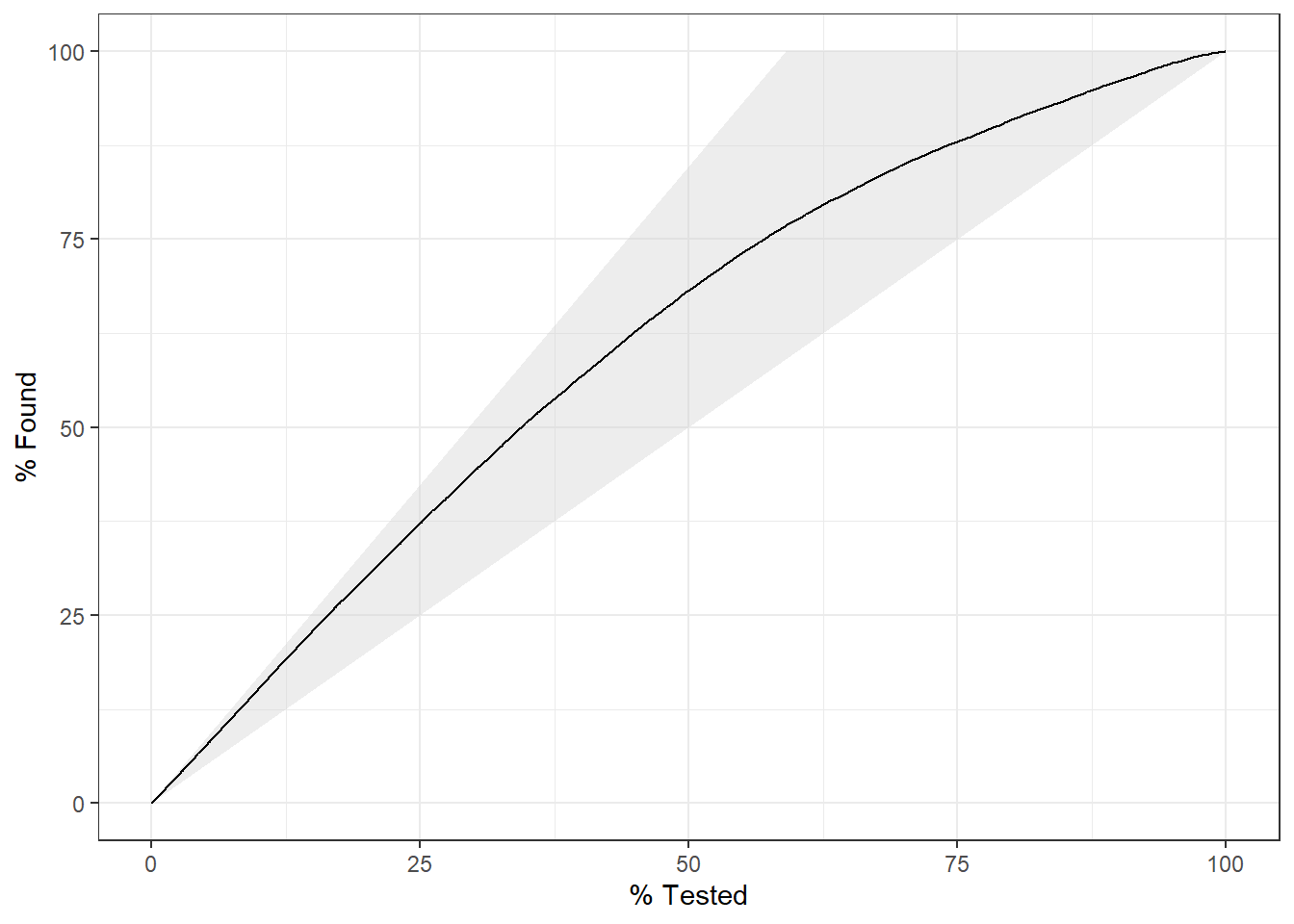
lift_curve:
pred_lm %>% lift_curve(truth = play_type, .pred_pass) %>%
  autoplot()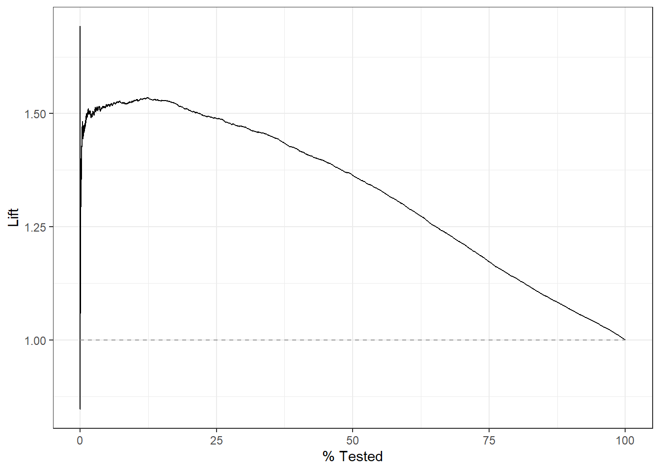
混淆矩阵:
pred_lm %>%
  conf_mat(play_type,.pred_class) %>%
  autoplot()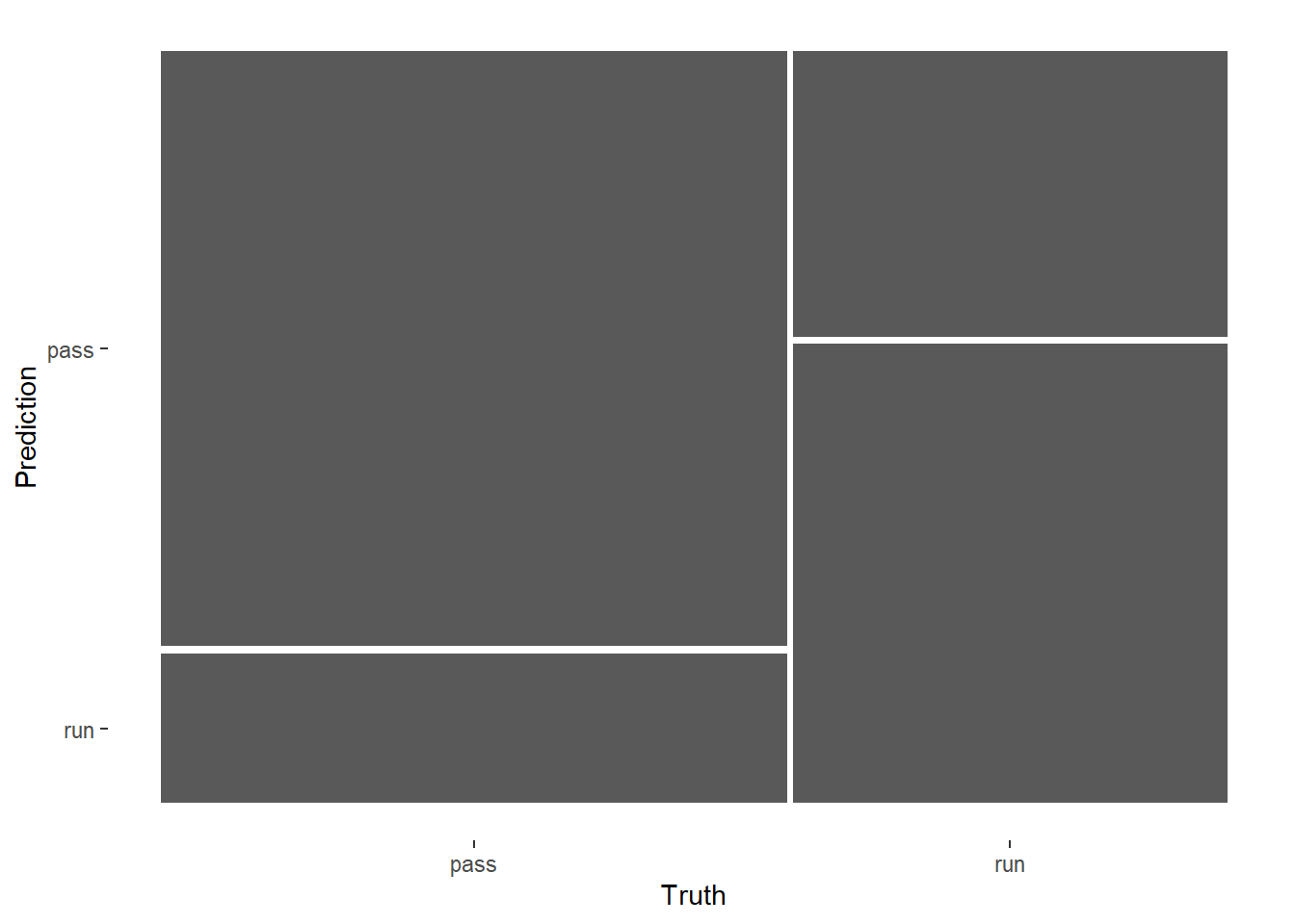
46.4.2 knn
k最近邻法,和上面的逻辑回归一模一样的流程。
首先也是选择模型,连接数据预处理步骤:
knn_spec <- nearest_neighbor(mode = "classification", engine = "kknn")

knn_wflow <- workflow() %>%
  add_recipe(pbp_rec) %>%
  add_model(knn_spec)
建立模型:
library(kknn)
fit_knn <- knn_wflow %>%
  fit(train_data)

#saveRDS(fit_knn,file = "datasets/fit_knn.rds")
应用于测试集:
pred_knn <- test_data %>% select(play_type) %>%
  bind_cols(predict(fit_knn, test_data, type = "prob")) %>%
  bind_cols(predict(fit_knn, test_data, type = "class"))
#saveRDS(pred_knn, file="./datasets/pred_knn.rds")
查看模型表现:
metricsets <- metric_set(accuracy, mcc, f_meas, j_index)

pred_knn %>% metricsets(truth = play_type, estimate = .pred_class)
## # A tibble: 4 × 3
##   .metric  .estimator .estimate
##   <chr>    <chr>          <dbl>
## 1 accuracy binary         0.672
## 2 mcc      binary         0.317
## 3 f_meas   binary         0.727
## 4 j_index  binary         0.315
pred_knn %>% roc_auc(play_type, .pred_pass)
## # A tibble: 1 × 3
## .metric .estimator .estimate
## <chr> <chr> <dbl>
## 1 roc_auc binary 0.718可视化模型的部分就不说了,和上面的一模一样!
46.4.3 随机森林
同样的流程来第3遍!
rf_spec <- rand_forest(mode = "classification") %>%
  set_engine("ranger",importance = "permutation")
rf_wflow <- workflow() %>%
  add_recipe(pbp_rec) %>%
  add_model(rf_spec)
建立模型:
fit_rf <- rf_wflow %>%
  fit(train_data)

#saveRDS(fit_rf,file = "datasets/fit_rf.rds")
应用于测试集:
pred_rf <- test_data %>% select(play_type) %>%
  bind_cols(predict(fit_rf, test_data, type = "prob")) %>%
  bind_cols(predict(fit_rf, test_data, type = "class"))
查看模型表现:
pred_rf %>% metricsets(truth = play_type, estimate = .pred_class)
## # A tibble: 4 × 3
##   .metric  .estimator .estimate
##   <chr>    <chr>          <dbl>
## 1 accuracy binary         0.731
## 2 mcc      binary         0.441
## 3 f_meas   binary         0.774
## 4 j_index  binary         0.439
pred_rf %>% conf_mat(truth = play_type, estimate = .pred_class)
## Truth
## Prediction pass run
## pass 10622 3226
## run 2962 6185pred_rf %>% roc_auc(play_type, .pred_pass)
## # A tibble: 1 × 3
## .metric .estimator .estimate
## <chr> <chr> <dbl>
## 1 roc_auc binary 0.799下面给大家手动画一个校准曲线。
两种画法,差别不大,主要是分组方法不一样,第2种分组方法是大家常见的哦~
calibration_df <- pred_rf %>%
   mutate(pass = if_else(play_type == "pass", 1, 0),
          pred_rnd = round(.pred_pass, 2)
          ) %>%
  group_by(pred_rnd) %>%
  dplyr::summarize(mean_pred = mean(.pred_pass),
            mean_obs = mean(pass),
            n = n()
            )

ggplot(calibration_df, aes(mean_pred, mean_obs))+
  geom_point(aes(size = n), alpha = 0.5)+
  geom_abline(linetype = "dashed")+
  theme_minimal()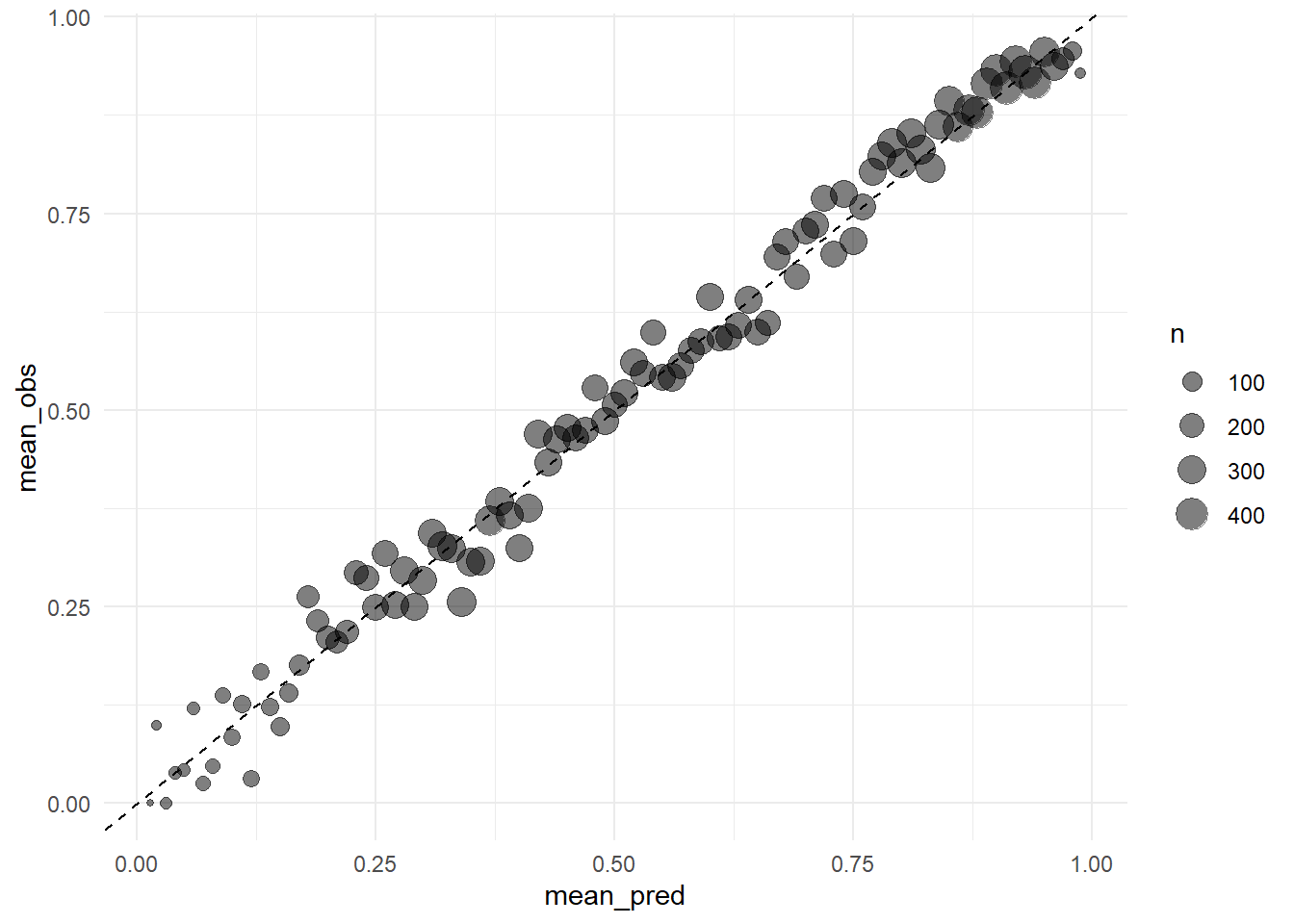
第2种方法:
cali_df <- pred_rf %>%
  arrange(.pred_pass) %>%
  mutate(pass = if_else(play_type == "pass", 1, 0),
         group = c(rep(1:249,each=92), rep(250,87))
         ) %>%
  group_by(group) %>%
  dplyr::summarise(mean_pred = mean(.pred_pass),
            mean_obs = mean(pass)
            )


cali_plot <- ggplot(cali_df, aes(mean_pred, mean_obs))+
  geom_point(alpha = 0.5)+
  geom_abline(linetype = "dashed")+
  theme_minimal()

cali_plot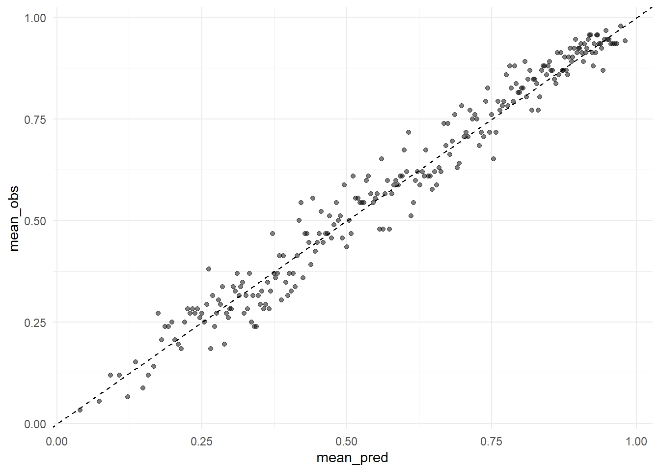
随机森林这种方法是可以计算变量重要性的,当然也是能把结果可视化的。
给大家演示下如何可视化随机森林结果的变量重要性:
library(vip)

fit_rf %>%
  extract_fit_parsnip() %>%
  vip(num_features = 10)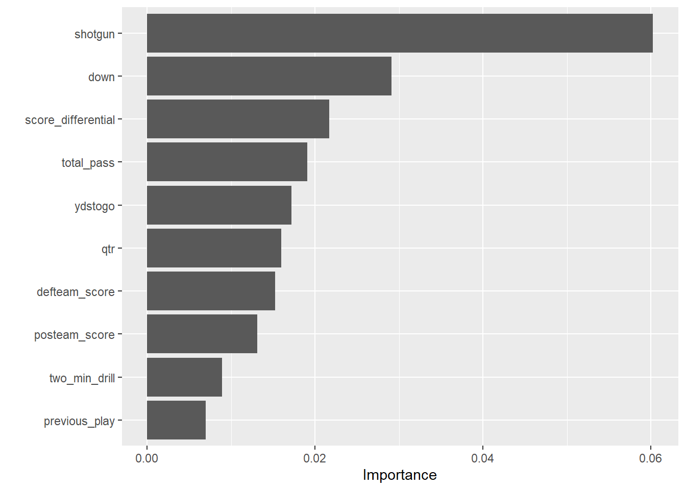
46.4.4 决策树
同样的流程来第4遍!不知道你看懂了没有。。。
tree_spec <- decision_tree(mode = "classification",engine = "rpart")
tree_wflow <- workflow() %>%
  add_recipe(pbp_rec) %>%
  add_model(tree_spec)
建立模型:
fit_tree <- tree_wflow %>%
  fit(train_data)
应用于测试集:
pred_tree <- test_data %>% select(play_type) %>%
  bind_cols(predict(fit_tree, test_data, type = "prob")) %>%
  bind_cols(predict(fit_tree, test_data, type = "class"))
查看结果:
pred_tree %>% roc_auc(play_type, .pred_pass)
## # A tibble: 1 × 3
##   .metric .estimator .estimate
##   <chr>   <chr>          <dbl>
## 1 roc_auc binary         0.706
pred_tree %>% metricsets(truth = play_type, estimate = .pred_class)
## # A tibble: 4 × 3
## .metric .estimator .estimate
## <chr> <chr> <dbl>
## 1 accuracy binary 0.721
## 2 mcc binary 0.417
## 3 f_meas binary 0.770
## 4 j_index binary 0.41146.5 交叉验证
交叉验证也是大家喜闻乐见的,就用随机森林给大家顺便演示下交叉验证。
首先要选择重抽样方法,这里我们选择10折交叉验证:
set.seed(20220520)

folds <- vfold_cv(train_data, v = 10)
folds
## #  10-fold cross-validation
## # A tibble: 10 × 2
##    splits               id
##    <list>               <chr>
##  1 <split [62082/6899]> Fold01
##  2 <split [62083/6898]> Fold02
##  3 <split [62083/6898]> Fold03
##  4 <split [62083/6898]> Fold04
##  5 <split [62083/6898]> Fold05
##  6 <split [62083/6898]> Fold06
##  7 <split [62083/6898]> Fold07
##  8 <split [62083/6898]> Fold08
##  9 <split [62083/6898]> Fold09
## 10 <split [62083/6898]> Fold10
然后就是让模型在训练集上跑起来:
keep_pred <- control_resamples(save_pred = T, verbose = T)

set.seed(20220520)

library(doParallel)

cl <- makePSOCKcluster(12) # 加速,用12个线程
registerDoParallel(cl)

rf_res <- fit_resamples(rf_wflow, resamples = folds, control = keep_pred)

stopCluster(cl)

#saveRDS(rf_res,file = "datasets/rf_res.rds")
查看模型表现:
rf_res %>%
  collect_metrics(summarize = T)
## # A tibble: 2 × 6
##   .metric  .estimator  mean     n std_err .config
##   <chr>    <chr>      <dbl> <int>   <dbl> <chr>
## 1 accuracy binary     0.732    10 0.00157 Preprocessor1_Model1
## 2 roc_auc  binary     0.799    10 0.00193 Preprocessor1_Model1
查看具体的结果:
rf_res %>% collect_predictions()
## # A tibble: 68,981 × 7
##    id     .pred_pass .pred_run  .row .pred_class play_type .config
##    <chr>       <dbl>     <dbl> <int> <fct>       <fct>     <chr>
##  1 Fold01      0.572    0.428      6 pass        pass      Preprocessor1_Model1
##  2 Fold01      0.470    0.530      8 run         pass      Preprocessor1_Model1
##  3 Fold01      0.898    0.102     22 pass        pass      Preprocessor1_Model1
##  4 Fold01      0.915    0.0847    69 pass        pass      Preprocessor1_Model1
##  5 Fold01      0.841    0.159     97 pass        pass      Preprocessor1_Model1
##  6 Fold01      0.931    0.0688   112 pass        pass      Preprocessor1_Model1
##  7 Fold01      0.727    0.273    123 pass        pass      Preprocessor1_Model1
##  8 Fold01      0.640    0.360    129 pass        pass      Preprocessor1_Model1
##  9 Fold01      0.740    0.260    136 pass        pass      Preprocessor1_Model1
## 10 Fold01      0.902    0.0979   143 pass        pass      Preprocessor1_Model1
## # ℹ 68,971 more rows
可视化结果也是和上面的一模一样,就不一一介绍了,简单说下训练集的校准曲线画法,其实也是和上面一样的~
res_calib_plot <- collect_predictions(rf_res) %>%
  mutate(
    pass = if_else(play_type == "pass", 1, 0),
    pred_rnd = round(.pred_pass, 2)
    ) %>%
  group_by(pred_rnd) %>%
  dplyr::summarize(
    mean_pred = mean(.pred_pass),
    mean_obs = mean(pass),
    n = n()
    ) %>%
  ggplot(aes(x = mean_pred, y = mean_obs)) +
  geom_abline(linetype = "dashed") +
  geom_point(aes(size = n), alpha = 0.5) +
  theme_minimal() +
  labs(
    x = "Predicted Pass",
    y = "Observed Pass"
    ) +
  coord_cartesian(
    xlim = c(0,1), ylim = c(0, 1)
    )

res_calib_plot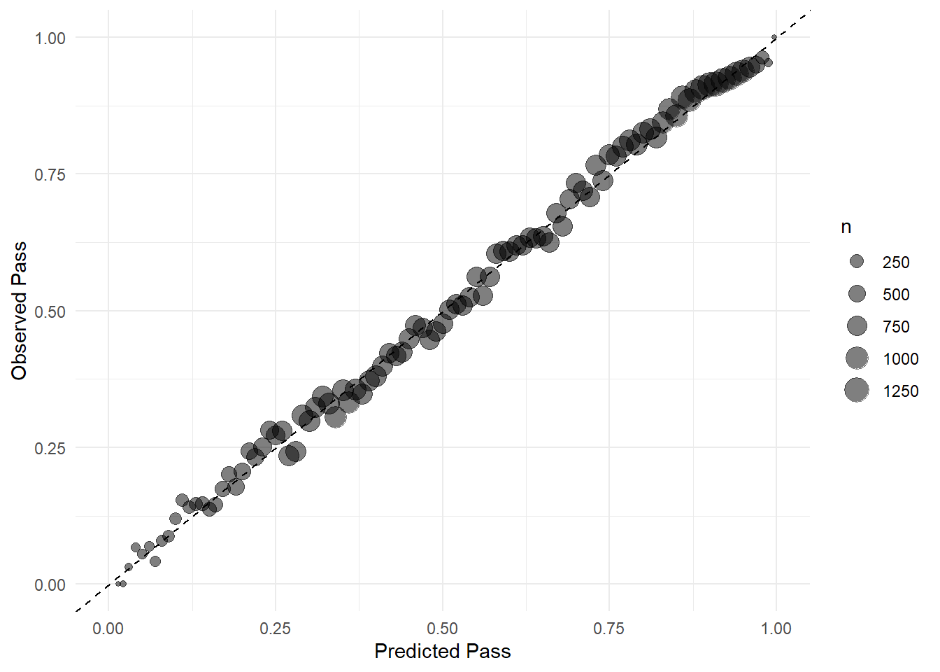
然后就是应用于测试集,并查看测试集上的表现:
rf_last_fit <- last_fit(rf_wflow, split_pbp)
#saveRDS(rf_last_fit,file = "./datasets/rf_last_fit.rds")
查看测试集表现:
rf_test_res <- rf_last_fit %>%
  collect_metrics()
rf_test_res
## # A tibble: 2 × 4
##   .metric  .estimator .estimate .config
##   <chr>    <chr>          <dbl> <chr>
## 1 accuracy binary         0.730 Preprocessor1_Model1
## 2 roc_auc  binary         0.799 Preprocessor1_Model1
多种指标:
metricsets <- metric_set(accuracy, mcc, f_meas, j_index)

collect_predictions(rf_last_fit) %>%
  metricsets(truth = play_type, estimate = .pred_class)
## # A tibble: 4 × 3
##   .metric  .estimator .estimate
##   <chr>    <chr>          <dbl>
## 1 accuracy binary         0.730
## 2 mcc      binary         0.439
## 3 f_meas   binary         0.774
## 4 j_index  binary         0.437
46.6 ROC曲线画一起
其实非常简单,就是把结果拼在一起画个图就行了~
roc_lm <- pred_lm %>% roc_curve(play_type, .pred_pass) %>%
  mutate(model = "logistic")

roc_knn <- pred_knn %>% roc_curve(play_type, .pred_pass) %>%
  mutate(model = "kknn")

roc_rf <- pred_rf %>% roc_curve(play_type, .pred_pass) %>%
  mutate(model = "randomforest")

roc_tree <- pred_tree %>% roc_curve(play_type, .pred_pass) %>%
  mutate(model = "decision tree")


rocs <- bind_rows(roc_lm,roc_knn,roc_rf,roc_tree) %>%
  ggplot(aes(x = 1 - specificity, y = sensitivity, color = model))+
  geom_path(lwd = 1.2, alpha = 0.6)+
  geom_abline(lty = 3)+
  coord_fixed()+
  scale_color_brewer(palette = "Set1")+
  theme_minimal()

rocs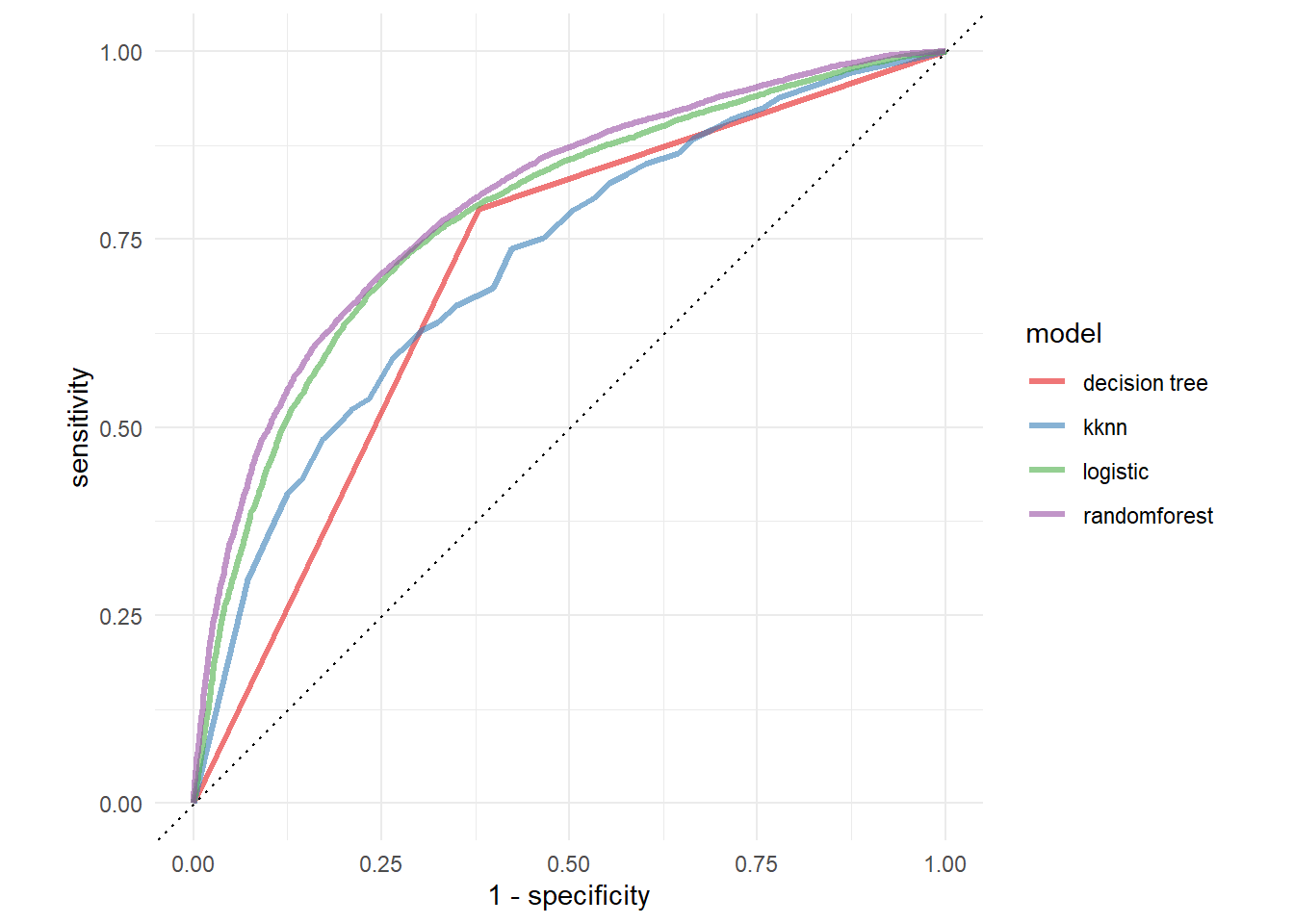
是不是很简单呢?二分类资料常见的各种评价指标都有了,图也有了,还比较了多个模型,一举多得,tidymodels,你值得拥有!